Set some env vars we need
Sys.setenv("AWS_NO_SIGN_REQUEST" = "YES")
Sys.setenv("AWS_S3_ENDPOINT" = "projects.pawsey.org.au")
Sys.setenv("AWS_VIRTUAL_HOSTING" = "FALSE")
library(sooty.watch)
watch_curated()
#> # A tibble: 24 × 4
#> Dataset mindate maxdate n
#> <chr> <dttm> <dttm> <int>
#> 1 ghrsst-tif 2002-06-01 00:00:00 2025-08-29 00:00:00 8491
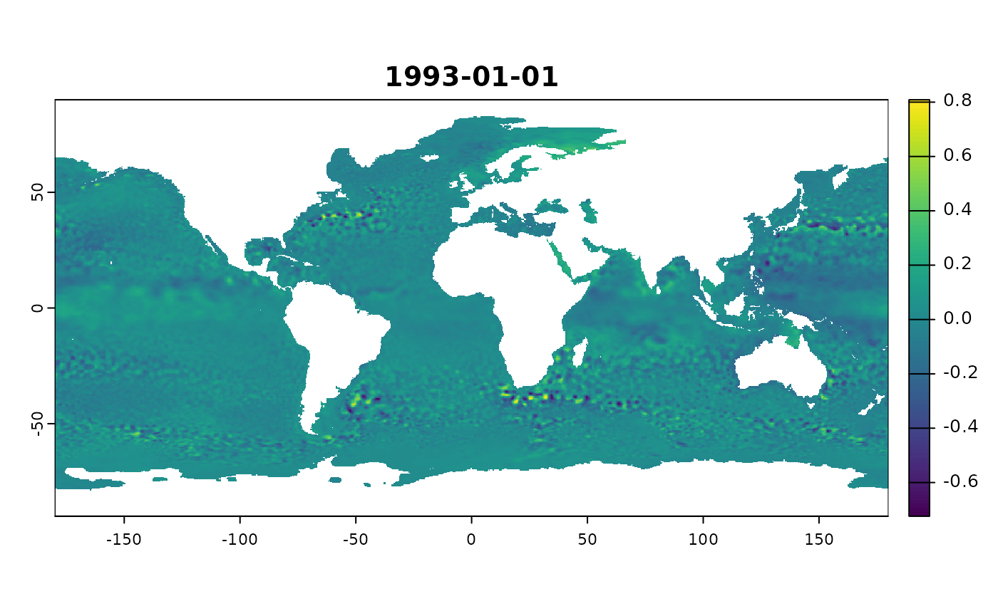
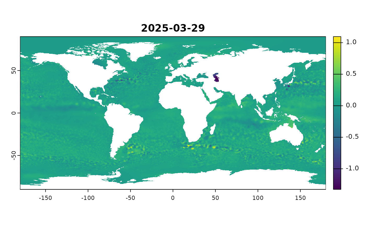
#> 2 SEALEVEL_GLO_PHY_L4 1993-01-01 00:00:00 2025-08-25 00:00:00 11811
#> 3 BREMEN-SEAICE-SMOS-north 2010-05-01 00:00:00 2025-08-24 00:00:00 5569
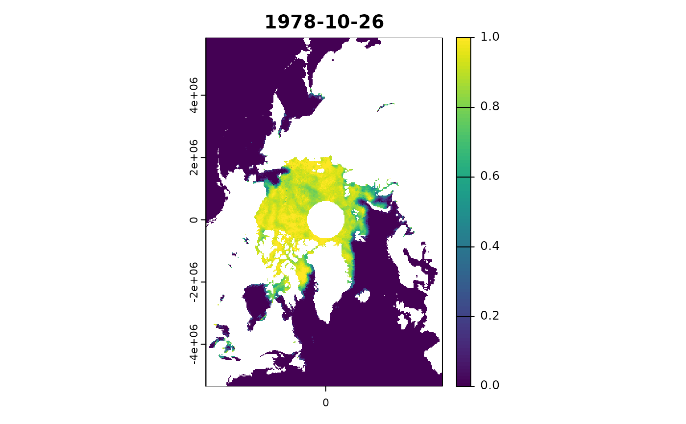
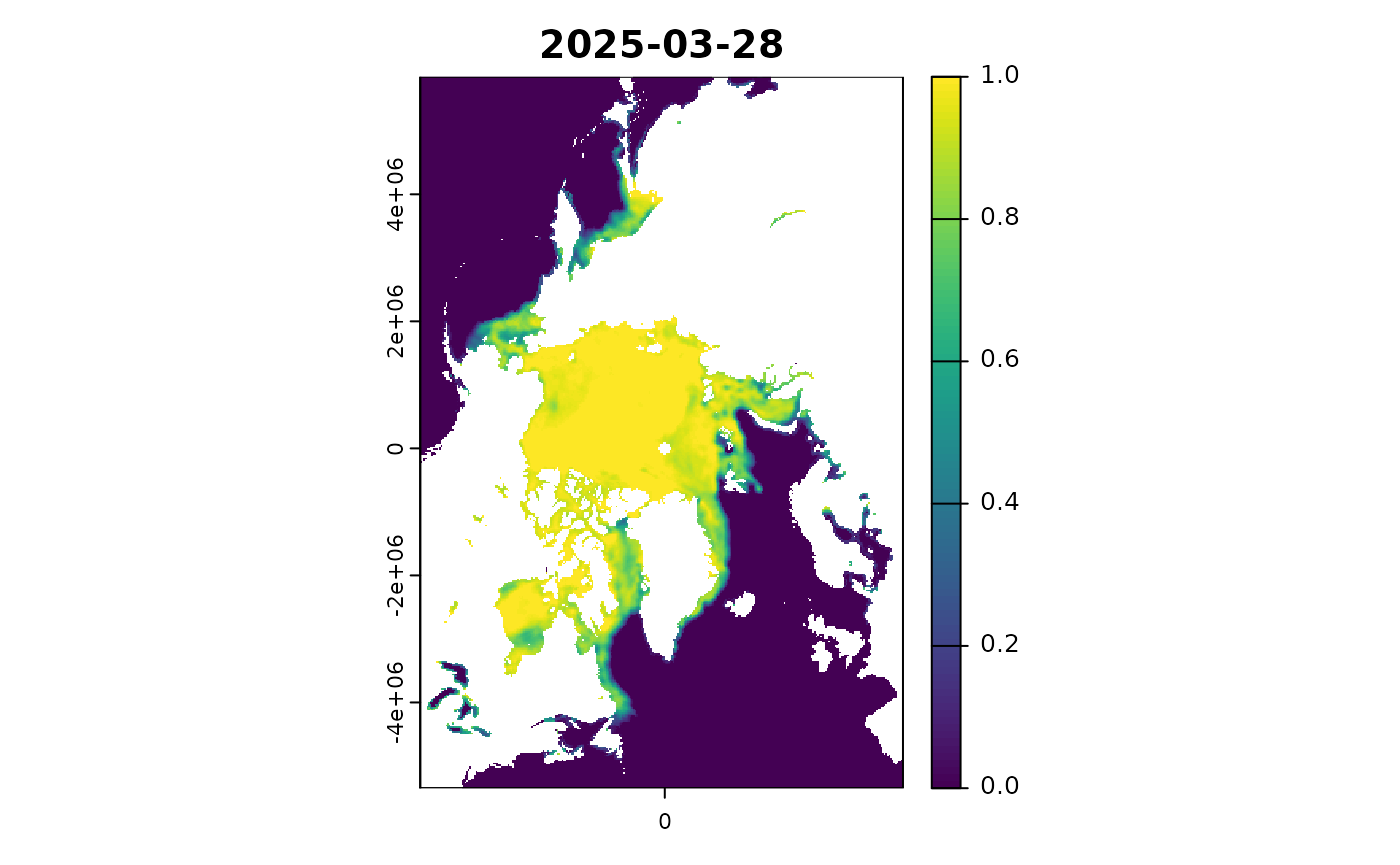
#> 4 NSIDC_SEAICE_PS_N25km 1978-10-26 00:00:00 2025-08-24 00:00:00 15448
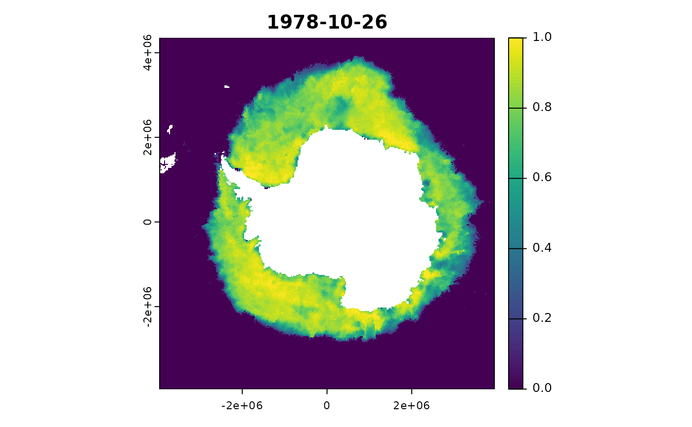
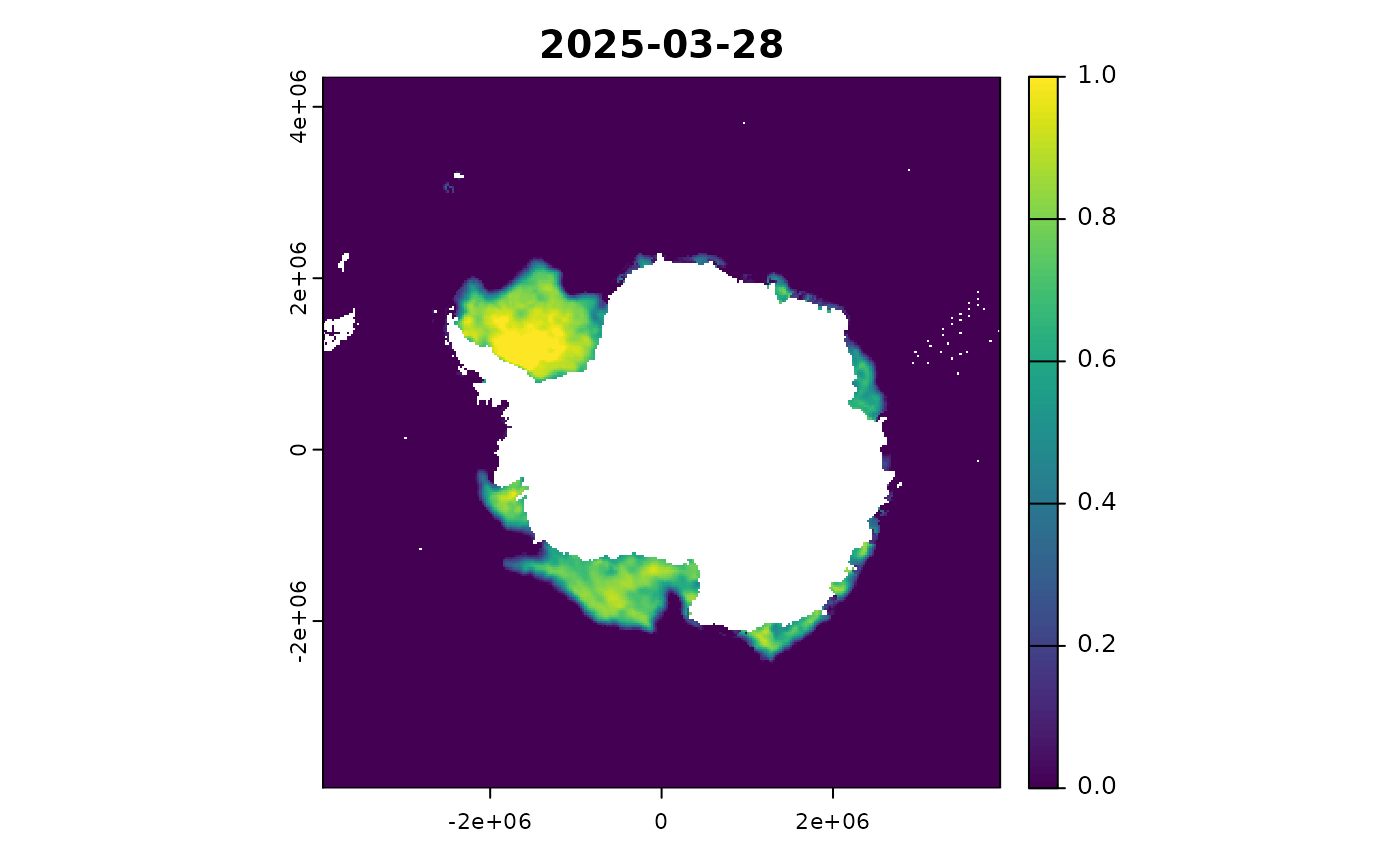
#> 5 NSIDC_SEAICE_PS_S25km 1978-10-26 00:00:00 2025-08-24 00:00:00 15448
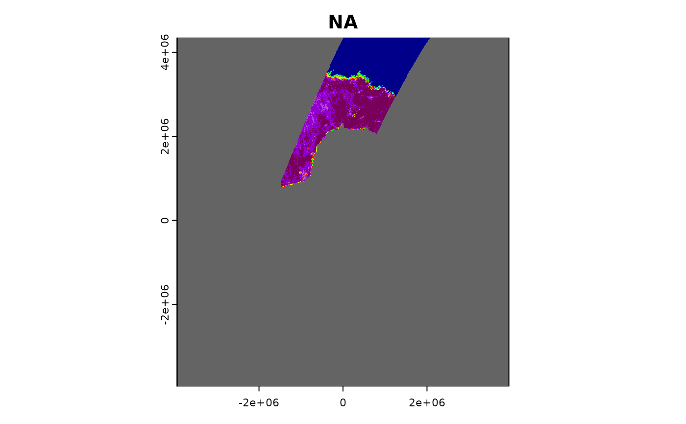
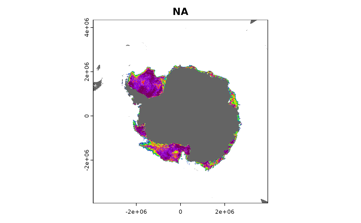
#> 6 antarctica-amsr2-asi-s3125-tif 2012-07-02 00:00:00 2025-08-24 00:00:00 4791
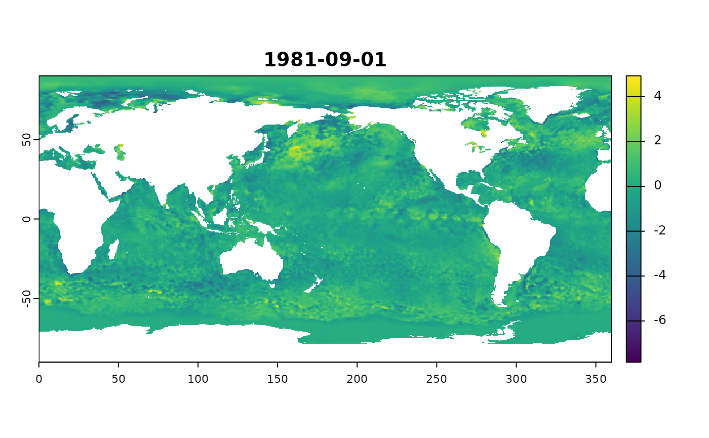
#> 7 oisst-avhrr-v02r01 1981-09-01 00:00:00 2025-07-17 00:00:00 16026
#> 8 sealevel-adt-tif 1993-01-01 00:00:00 2025-05-23 00:00:00 11717
#> 9 sealevel-err_sla-tif 1993-01-01 00:00:00 2025-05-23 00:00:00 11717
#> 10 sealevel-err_ugosa-tif 1993-01-01 00:00:00 2025-05-23 00:00:00 11717
#> # ℹ 14 more rows
watch_buckets()
#> # A tibble: 10 × 2
#> Bucket n
#> <chr> <int>
#> 1 sealevel-glo-phy-tif 117170
#> 2 idea-10.5067-mpyg15waa4wx 30896
#> 3 idea-10.7289-v5sq8xb5 16026
#> 4 idea-oisst 14057
#> 5 idea-esacci 12423
#> 6 ccmp-wind-product-v2 11552
#> 7 idea-sealevel-glo-phy-l4-rep-observations-008-047 11208
#> 8 idea-amsr2-asi-s3125 10372
#> 9 ausantarctic 8491
#> 10 idea-sealevel-glo-phy-l4-nrt-008-046 603For each dataset, let’s get the first and last and plot.
library(dplyr)
datasets <- group_by(sooty::sooty_files(), Dataset)
th <- function(x, ...) rbind(head(x, 1L), tail(x, 1L))
read1 <- function(x) {
out <- terra::rast(x)[[1]]
names(out) <- substr(names(out), 1, 24)
out
}
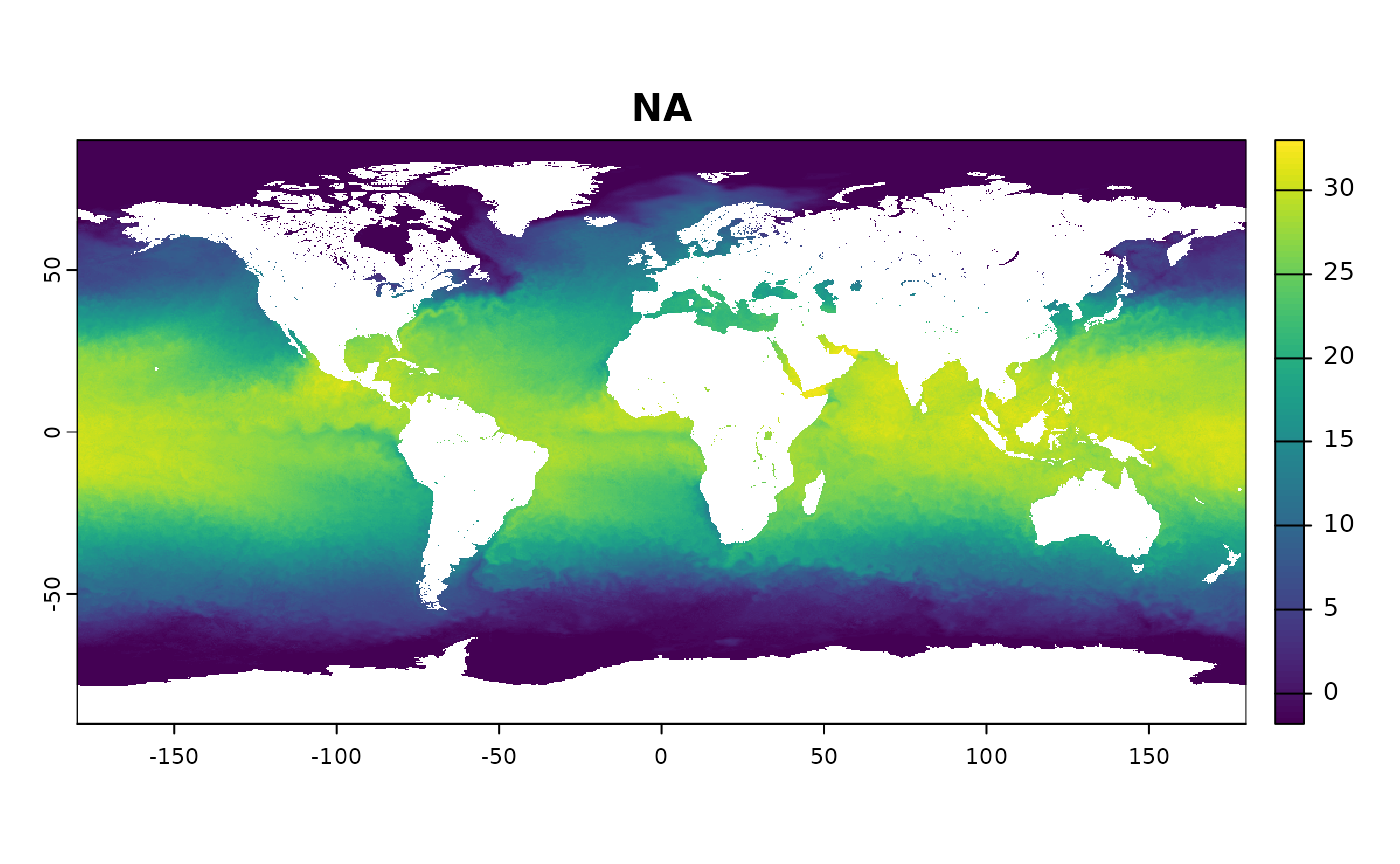
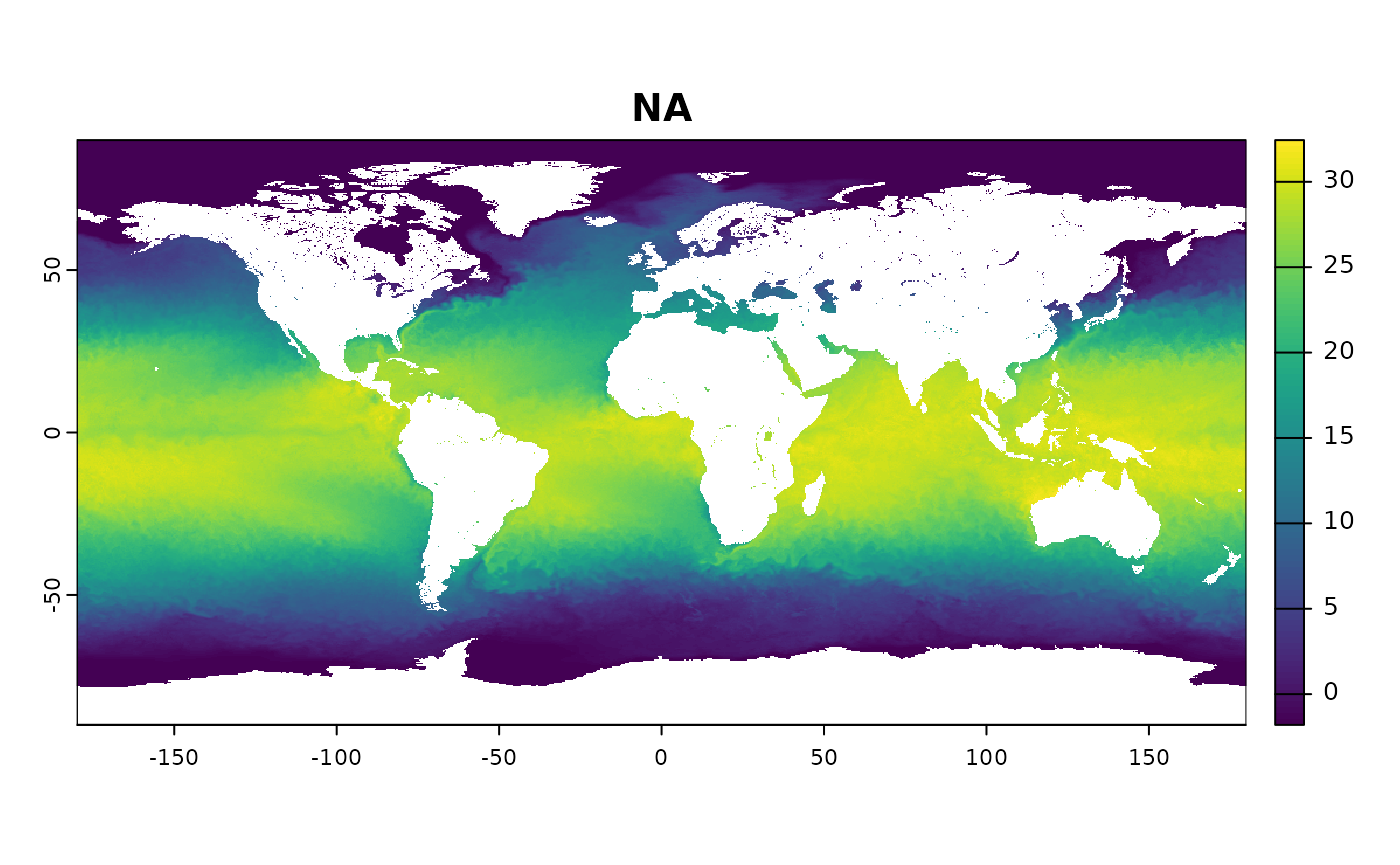
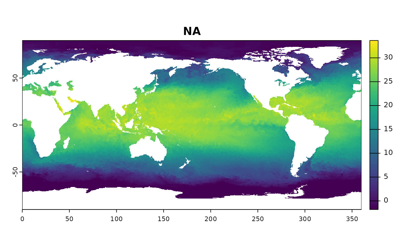
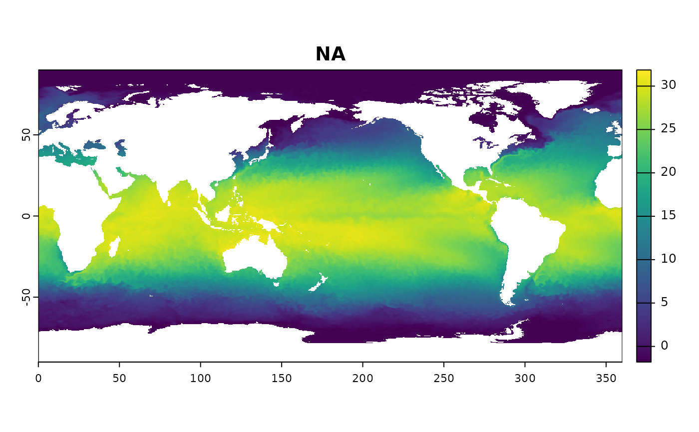
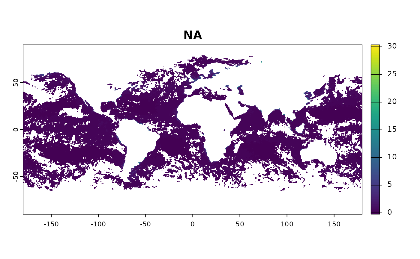
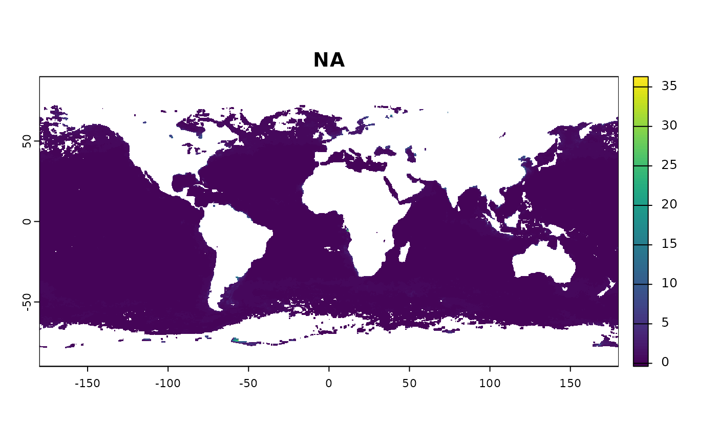
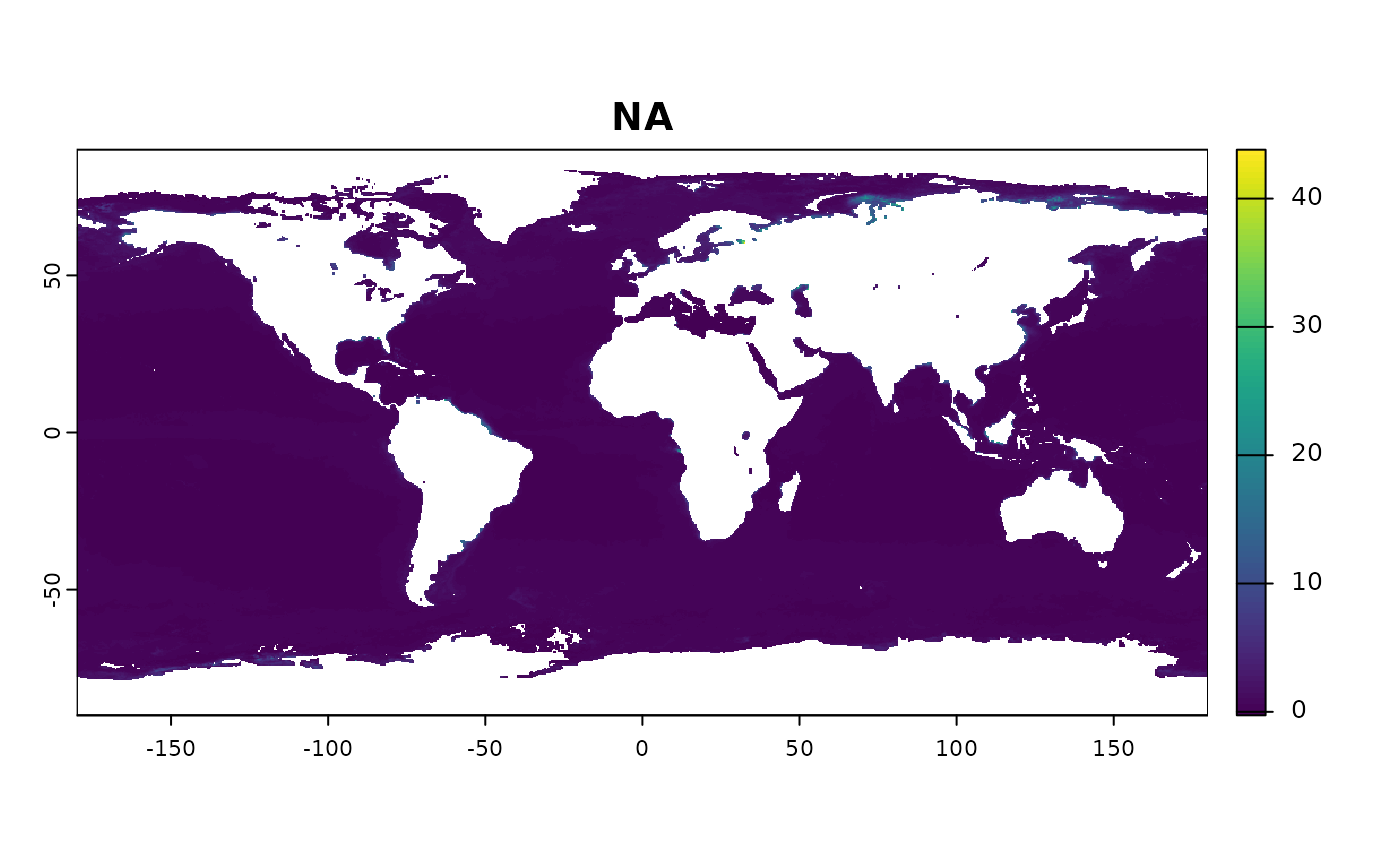
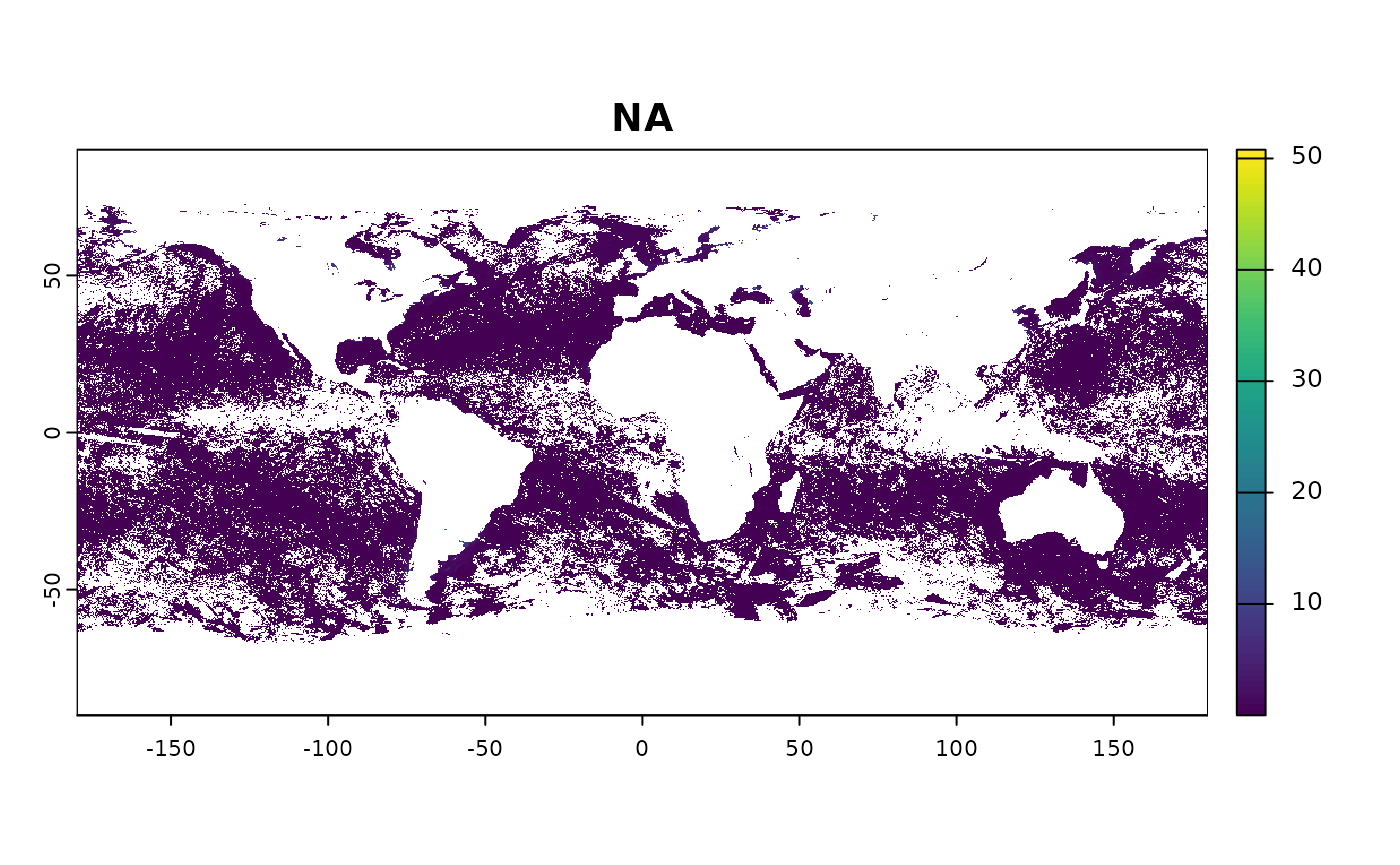
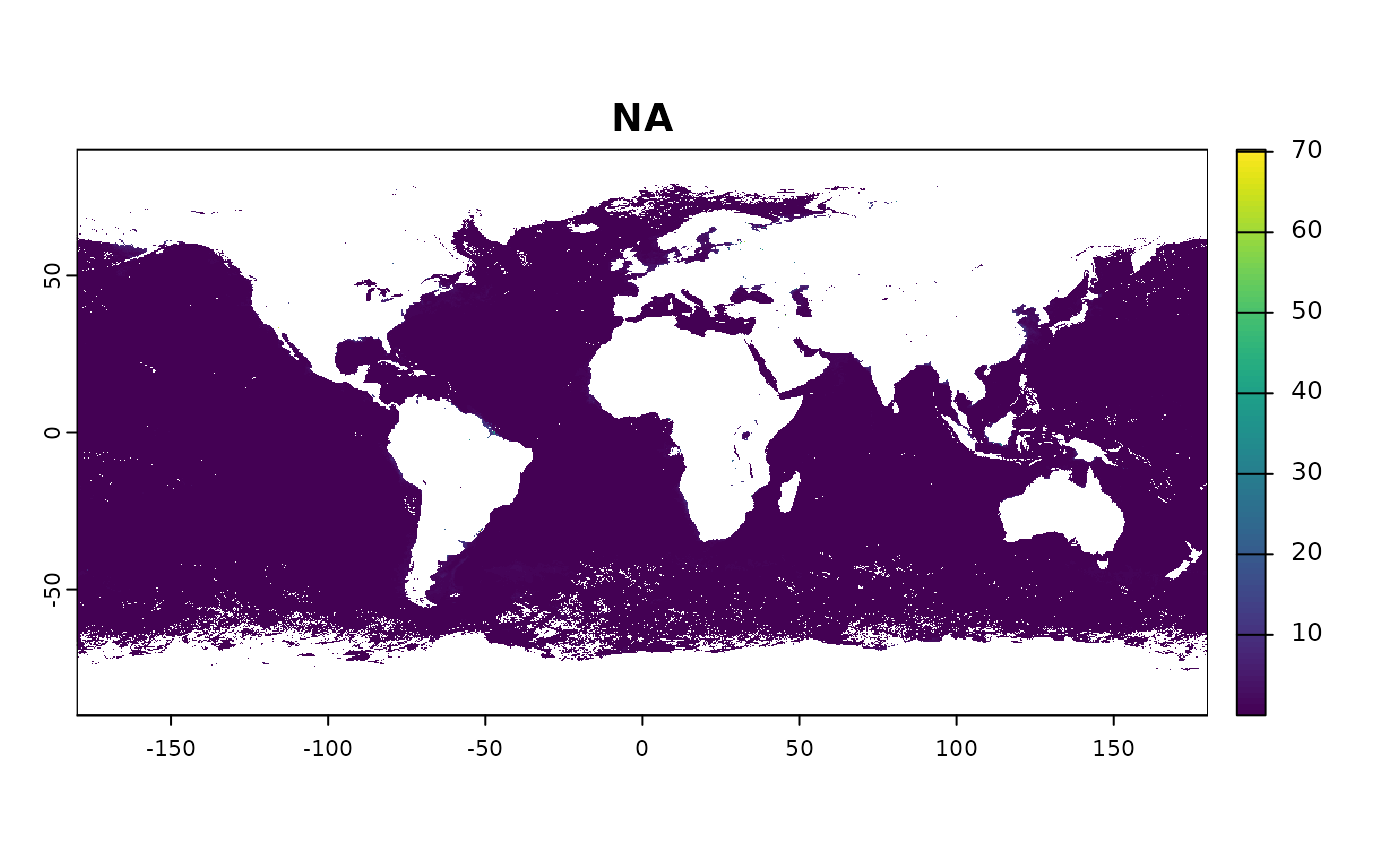
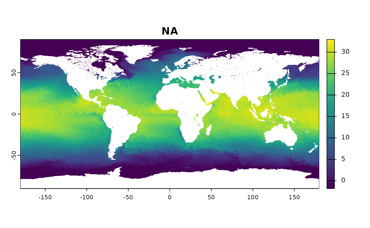
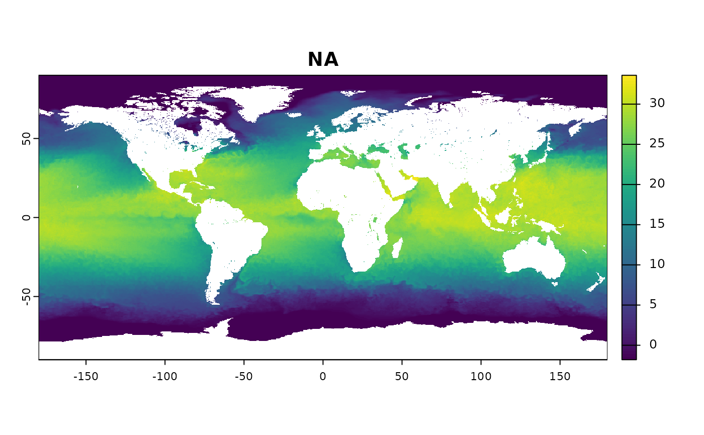
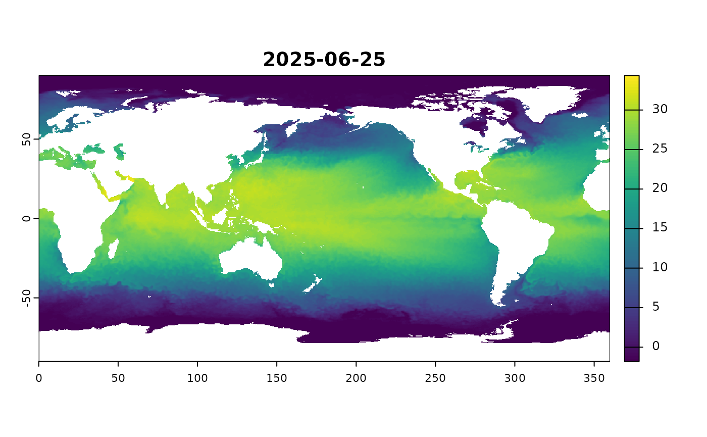
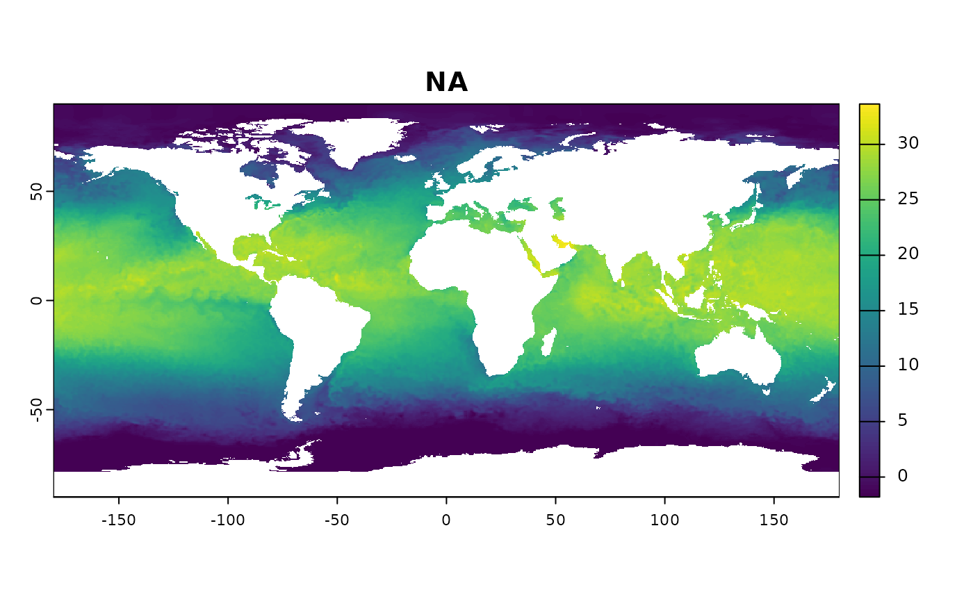
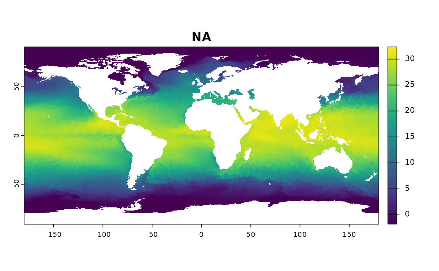
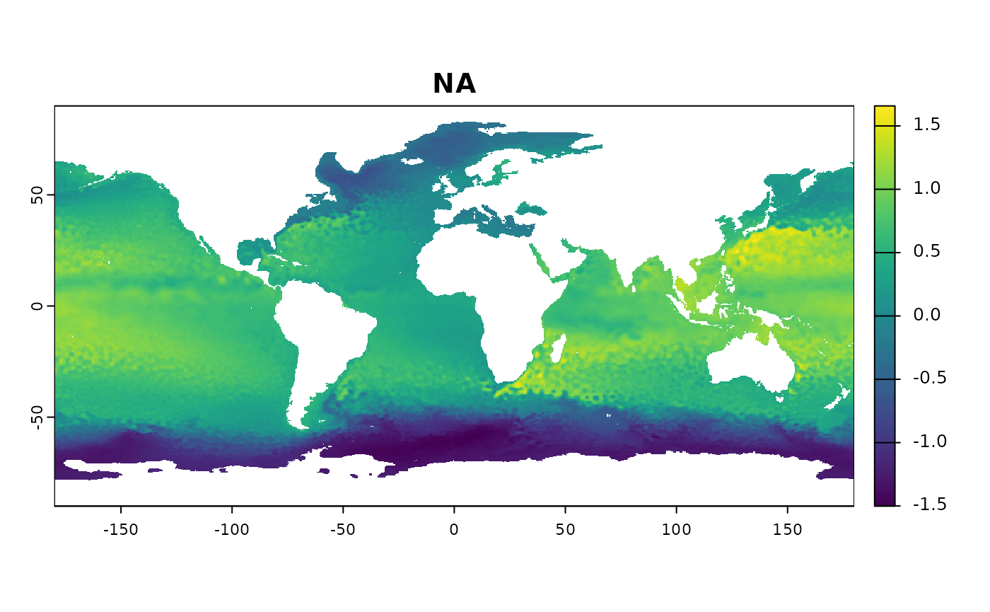
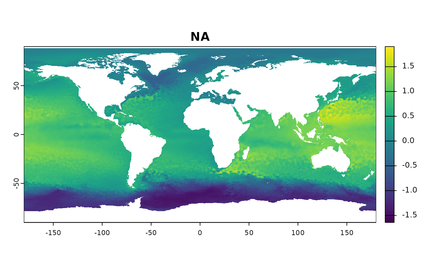
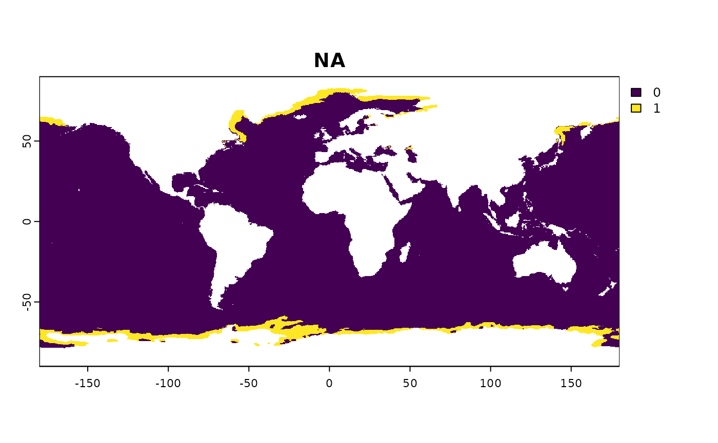
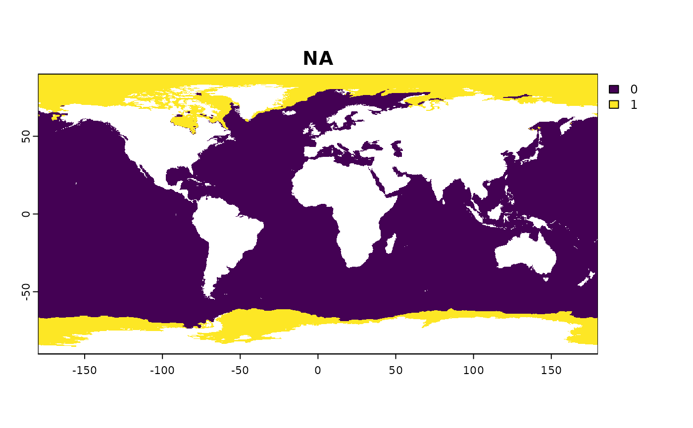
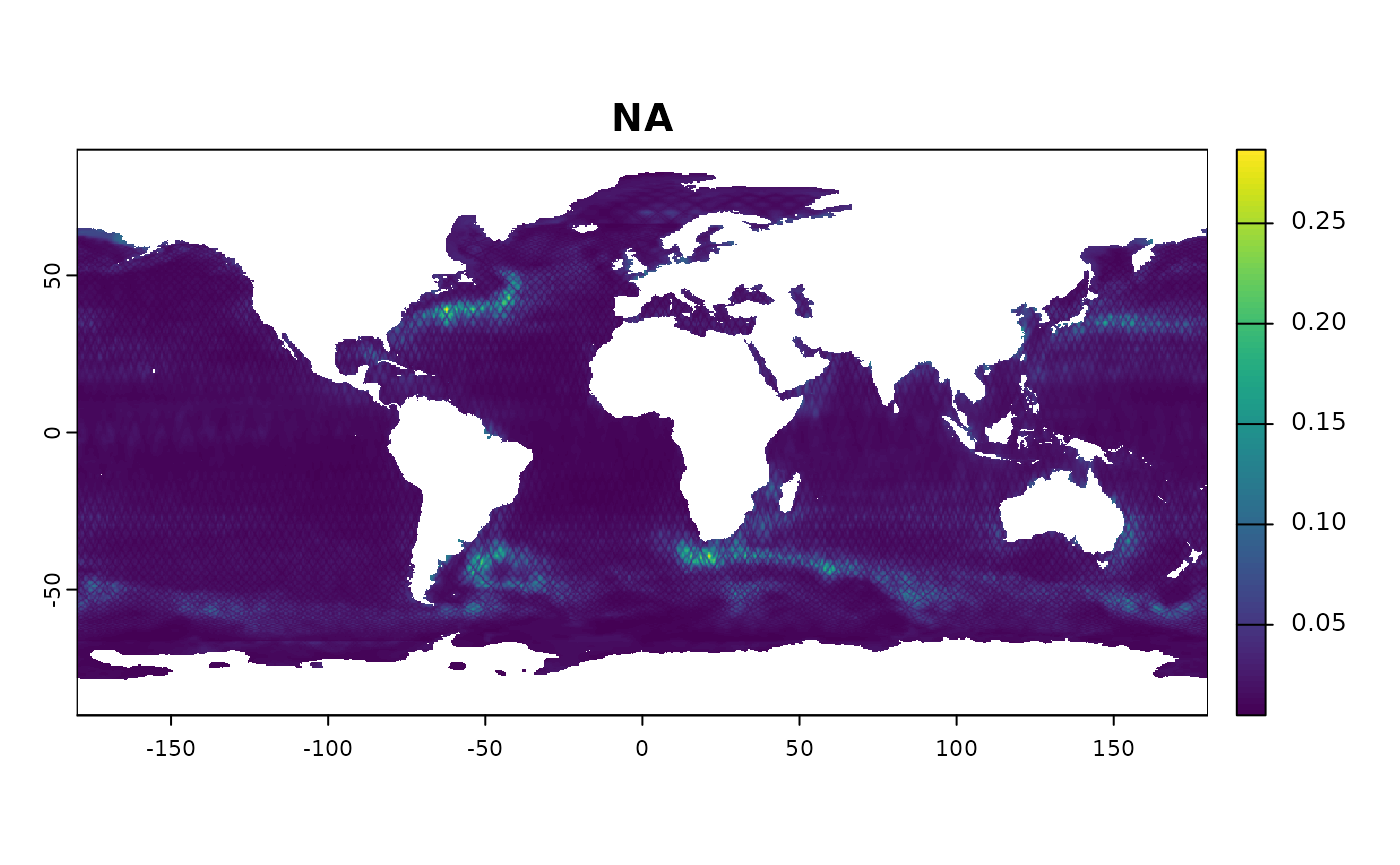
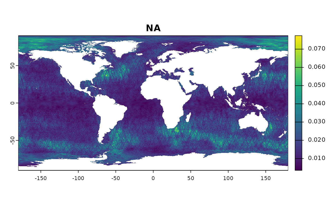
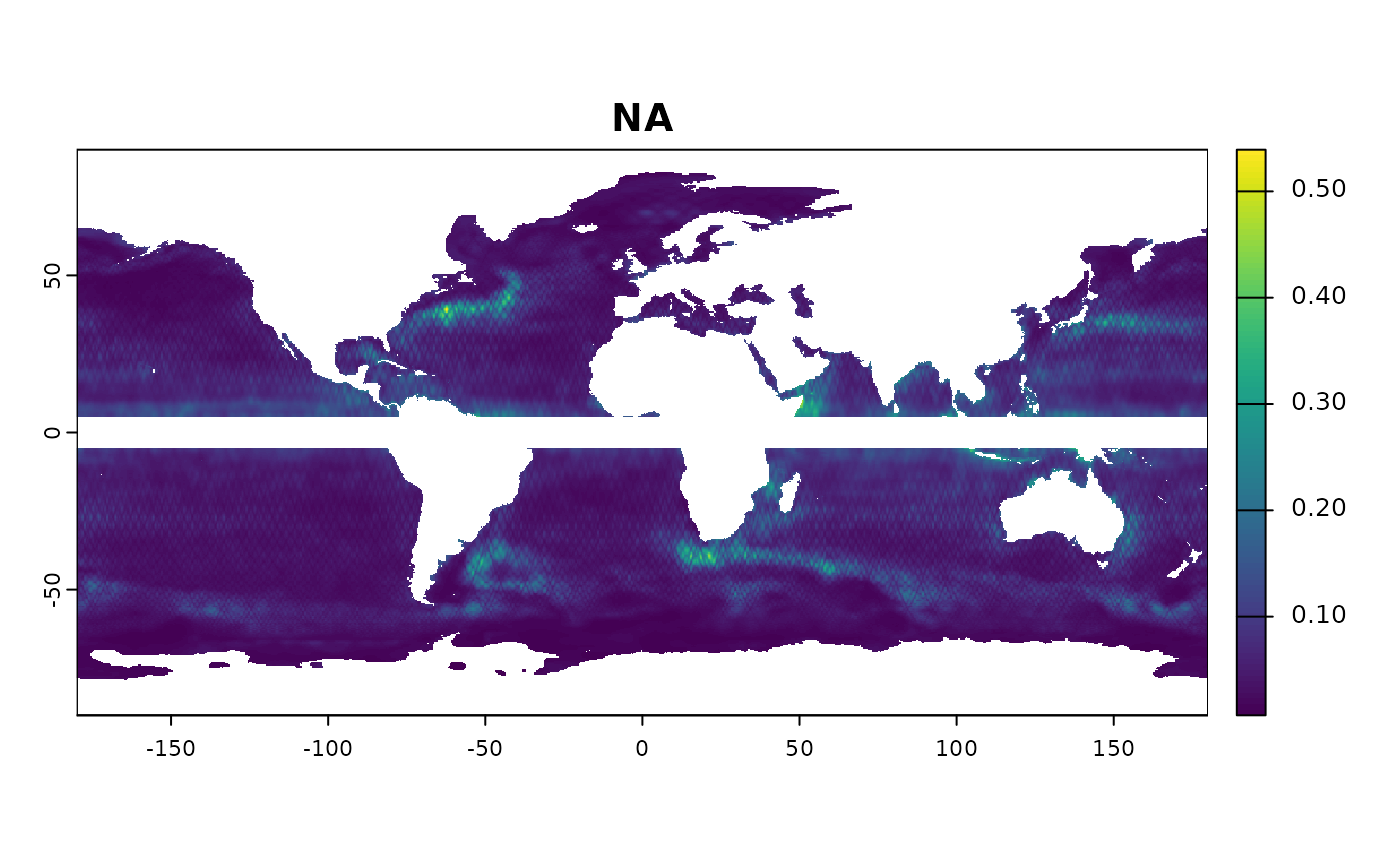
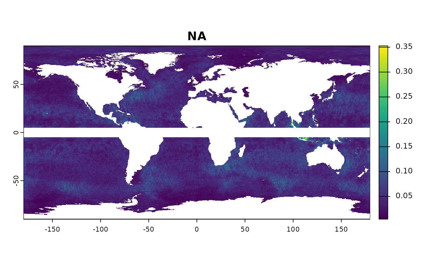
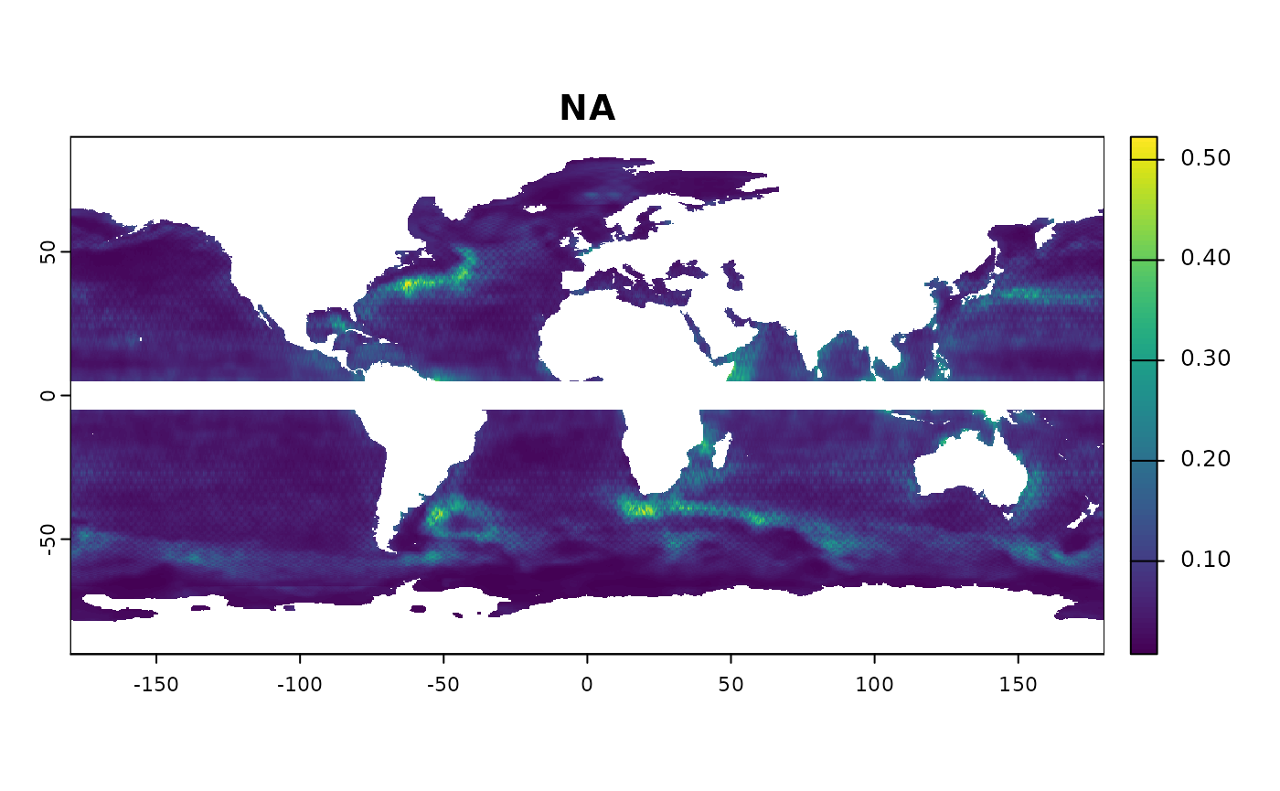
plotfun <- function(x) {
plot(x[[1]], main = format(time(x[[1]]))); plot(x[[2]], main = format(time(x[[2]])))
}
library(terra)
#> terra 1.9.1
ctch <- dplyr::group_map(datasets, \(.x, ...) try(plotfun(lapply(th(.x)$source, read1))))