Chapter 4 The mesh3d format
Rgl is the OpenGL package in R.
A classic computer graphics data model called mesh3d, it’s not widely used but is very powerful. You can visualize a mesh3d model with shade3d(), all the aesthetics, material properties, geometry and topology can be attached to the model
itself as data.
It supports two kinds of primitives quads and triangles.
4.1 Quads
Quads are a funny case, usually carried by two triangles (at least implicitly) but they are an important computer graphics element.
Previously, we created a raster with effectively the following code.
m <- matrix(c(seq(0, 0.5, length = 5),
            seq(0.375, 0, length = 4)), 3)

x <- seq(1, nrow(m)) - 0.5
y <- seq(1, ncol(m)) - 0.5
rast <- raster::raster(list(x = x, y = y, z = m))
If we convert that to a quadmesh, the result has vertices (vb) and primitives (ib).
## List of 8
##  $ vb             : num [1:4, 1:16] 0 3 0.312 1 1 ...
##   ..- attr(*, "dimnames")=List of 2
##   .. ..$ : chr [1:4] "x" "y" "z" "1"
##   .. ..$ : NULL
##  $ ib             : int [1:4, 1:9] 1 2 6 5 2 3 7 6 3 4 ...
##  $ primitivetype  : chr "quad"
##  $ material       : list()
##  $ normals        : NULL
##  $ texcoords      : NULL
##  $ raster_metadata:List of 7
##   ..$ xmn  : num 0
##   ..$ xmx  : num 3
##   ..$ ymn  : num 0
##   ..$ ymx  : num 3
##   ..$ ncols: int 3
##   ..$ nrows: int 3
##   ..$ crs  : chr "+proj=longlat +datum=WGS84 +ellps=WGS84 +towgs84=0,0,0"
##  $ crs            : chr "+proj=longlat +datum=WGS84 +ellps=WGS84 +towgs84=0,0,0"
##  - attr(*, "class")= chr [1:3] "quadmesh" "mesh3d" "shape3d"
The structure is vb, the coordinates of the mesh - these are the
actual corner coordinates from the input raster.
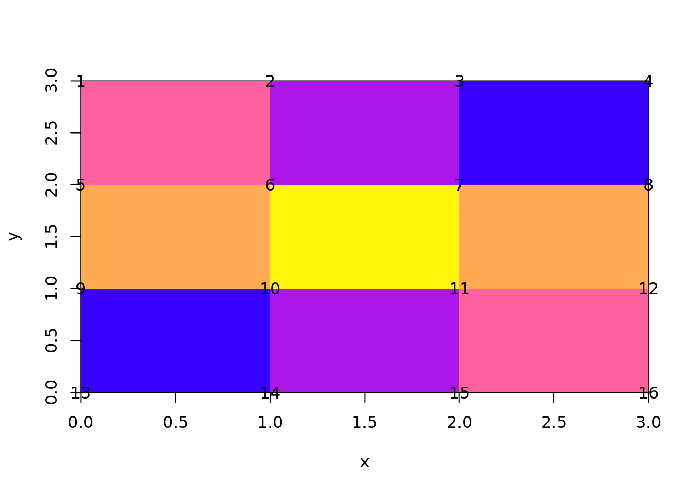
Notice how these are unique coordinates, there’s no simple relationship between the cell and its value and its four corners. This is because they are shared between neighbouring cells. The relationship is stored in the ib array, this has four rows one for each corner of each cell. There are 9 cells and each has four coordinates from the shared vertex pool. The cells are defined in the order they occur in raster.
##      [,1] [,2] [,3] [,4] [,5] [,6] [,7] [,8] [,9]
## [1,]    1    2    3    5    6    7    9   10   11
## [2,]    2    3    4    6    7    8   10   11   12
## [3,]    6    7    8   10   11   12   14   15   16
## [4,]    5    6    7    9   10   11   13   14   15
It works directly with rgl function, and can be used in more raw form.
They key point in these plots is that with the exact same 3D geometry, we have the choice of how each primitive is styled. The colour may be a constant every where, or it may vary continuously everywhere between vertices. A final choice is that the colour is constant within a primitive. No R 2D plot can easily do the continuous texture styling. This also applies to other kinds of textures, later we will apply an image texture to primitives.
The situation for triangles is much the same, but we have it for the triangle index rather than ib for the quad index. In both cases the geometry is in the vb matrix. Models can have both quads and triangles, using the same set of vertices.
4.2 Triangles
Triangles aren’t so readily created, although it is easy to convert a quadmesh version of a raster into triangles.
For polygons, we need specialist code. There are two algorithm types:
- ear-clipping (or ear-cutting)
- near-Delaunay methods
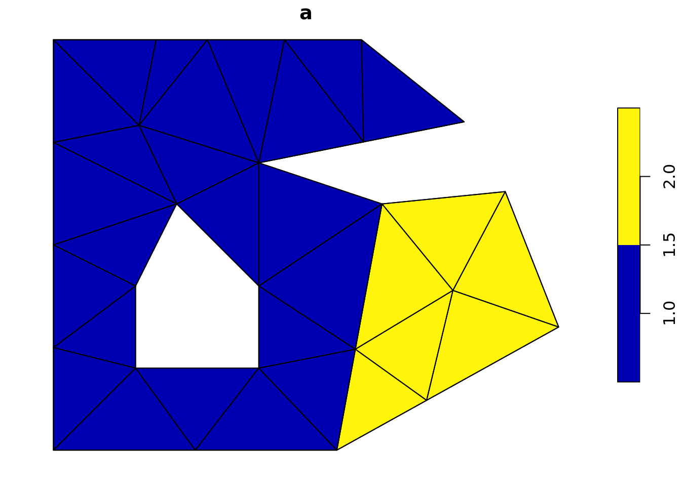
The mesh_polys object is create from the two_polys simple features layer using ear-clipping.
This is a very simple algorithm, it chooses one corner of the polygon and clips off a triangle at the next vertex, then proceeds around the boundary - the decido package on CRAN uses the Mapbox library earcut to do this.

The delaunay_polys object is created from two_polys using the in-development anglr package, on Github only - anglr uses the RTriangle package from CRAN to do this. All edges in the polygons are fed to the algorithm which creates all constrained triangles, then this mesh of triangles is processed to determine which polygon (or hole) each belongs to. With RTriangle we can also specify properties like maximum triangle area, or “conform to Delaunay criterion”. (This is why we always call polygon triangulation near-Delaunay …).
This mesh is both Delaunay-conforming and applying a maximum triangle area, so extra vertices have been added that weren’t in the original polygons.
4.3 3D polygons
If we don’t have triangles (or quads), we can’t plot surfaces or polygons in 3D at all.
But, unless we modify the material properties of the surface, or update the geometry in the 3rd dimension we cannot tell the difference between these different mesh polygons.
Let’s push the Delaunay version up in Z and add some noise.
clear3d()
delaunay_polys$vb[3,] <- 0
delaunay_polys$vb[3,] <- delaunay_polys$vb[3,] +
    runif(ncol(delaunay_polys$vb), 1, 1.5)
wire3d(mesh_polys, col = "grey")
wire3d(delaunay_polys)
rglwidget()
The primary means to create this format from a raster is for 3D plotting, but because we have access to the coordinate directly it provides other uses. We can transform the coordinates (i.e. a map projection) or manipulate them and augment the Z value (for example) in flexible ways.
(The usual way of driving rgl grid surfaces is rgl.surface but this is limited to the centre-point interpretation only - more than the x, y, z list interface as image() is, i.e. it can take an individual x,y pair for every cell, but it cannot properly represent the cell-as-area as image can. For this we need to use shade3d, and actual meshd3d types in rgl).
4.4 rgl miscellanea
Most examples around use rgl.surface, but I am less familiar with that. The thing3d() are the higher-level functions in rgl, and the rgl.thing() functions are lower-level (recommended not to mix them in usage).
rayshader in particular, has extremely compelling outputs, but it uses the lower level rgl.surface and doesn’t maintain the geographic coordinates, so I see it mostly as a texture-generator (but watch its development!).
rgl.surface can take X and Y matrices, so you can trivially reproject these data and wrap them around a sphere - I only learnt this recently.
WATCH OUT
The single most confusing thing I found with mesh3d was homogeneous coordinates. This is a fourth value on each vertex, making it X, Y, Z, H and because it’s stored transpose, the ib and the vb matrices have the same number of rows (4). The H loosely corresponds to “zoom”, for our purposes set H = 1. (If set to 0 no data will be visible, and a package of mine had this bug until last week.)