2  R and image

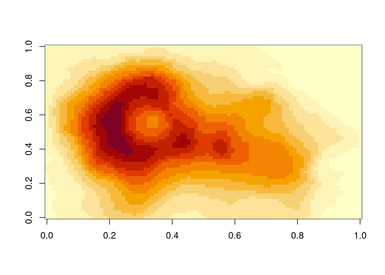
Base R has since at least 1998 had the volcano dataset (a 61x87 matrix of integer heights from Mauna Whau) and the image() function.

The image() function takes matrix and draws it by mapping a numerical value in matrix elements to a colour intensity on the screen.

image(volcano)

No georeferencing information is included with the dataset other than that it was hand digitized from a map and that the pixel size is 10m either side. So in this plot there is 870 in the x direction, and 610m in the y direction but here image() defaults to the unit square (which is shame because we have lost all sense of the aspect ratio). Also if you know what Mauna Whau usually looks like on a north-up map you’ll know that it seems rotated (90 degrees clockwise) from that.

We know that the dataset has extent 2667400, 2668010, 6478700, 6479570 (xmin, xmax, ymin, ymax) on New Zealand Map Grid (NZGD49 / New Zealand Map Grid (EPSG:27200)).

To plot with image() we must generate the 1D-coord arrays that position the matrix in this extent.

ex <- c(2667400, 2668010, 6478700, 6479570)
xs <- seq(ex[1L], ex[2L], length.out = 61L + 1L)
ys <- seq(ex[3L], ex[4L], length.out = 87L + 1L)
image(xs, ys, t(volcano[,  61:1]), asp = 1)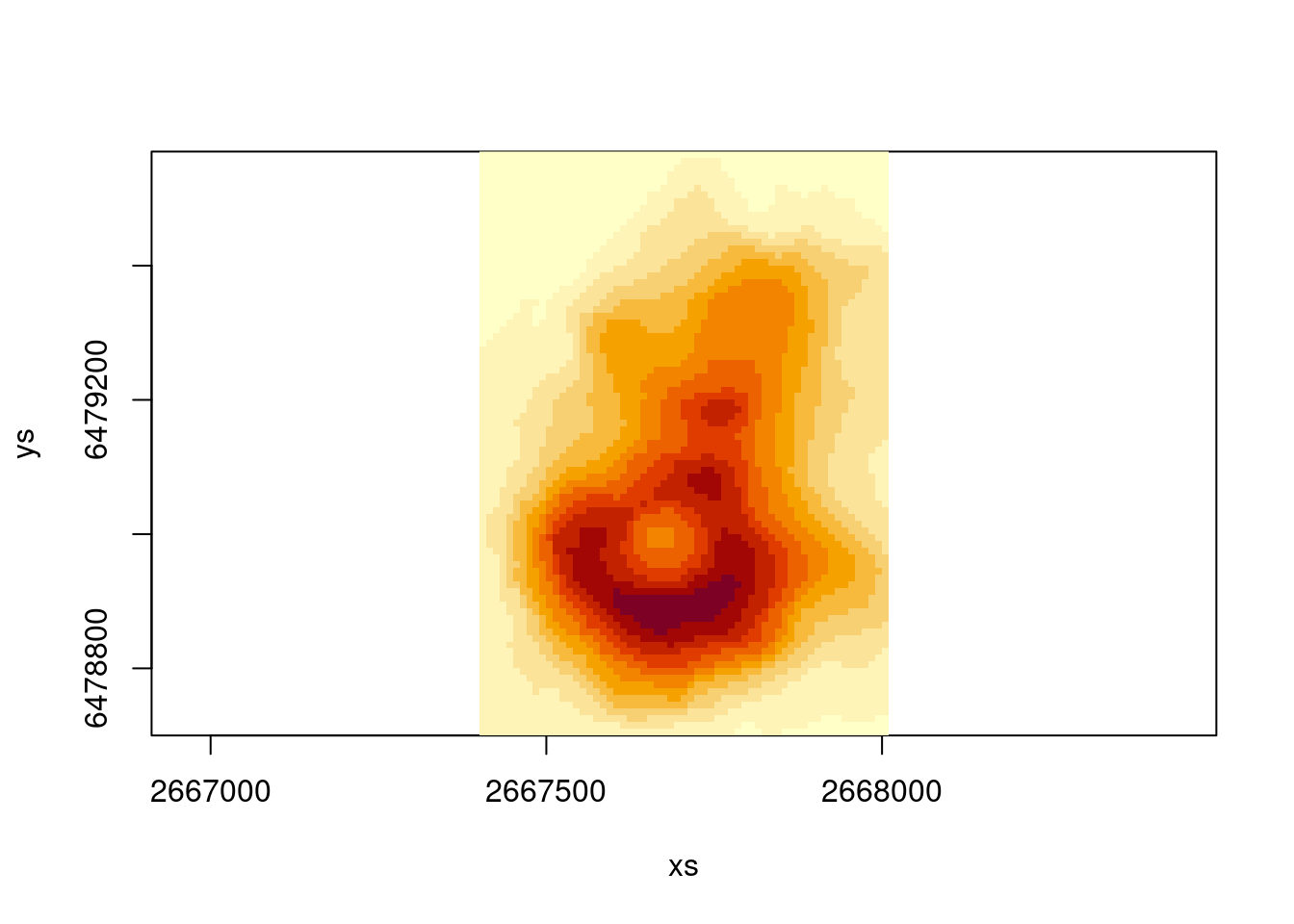

We know this is correct, but we’ll prove it also by obtaining some imagery data from online and overplotting our volcano dataset.

library(ximage)
library(whatarelief)
im <- imagery(extent = ex, dimension = c(610L, 870L), projection = "EPSG:27200")
ximage(im, ex, asp = 1)
xc <- xs[-length(xs)] + diff(xs[1:2])/2
yc <- ys[-length(xs)] + diff(ys[1:2])/2
contour(xc, yc, t(volcano[,  61:1]), add = TRUE, col = "hotpink")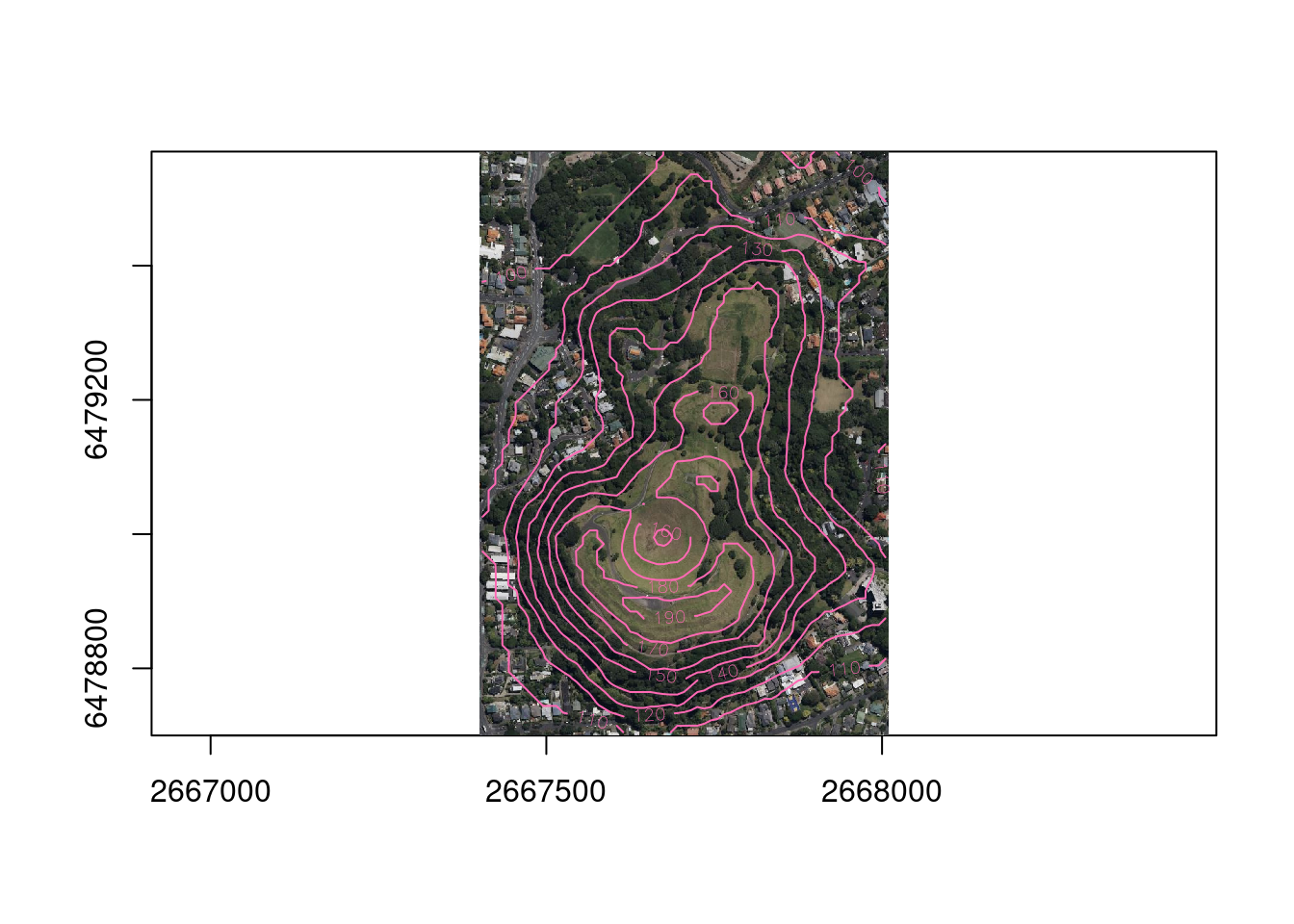

Note here that we have had to convert from referencing to the edges of the pixels to referencing to the centres for using contour. This is an inconsistency deep in R itself, and is just one example of the complex of problems that inspired the topic of this book.