
Installation
Install from CRAN with
install.packages("ozmaps")The development version of ozmaps may be installed directly from github.
devtools::install_github("mdsumner/ozmaps")The package includes some simple features data, which can be used independently of ozmaps with the sf package. If required, install sf from CRAN.
NOTE: Since April 2020) we must have sf installed because of requirements of the tibble package.
If sf causes you problems or you can’t work with it get in touch and I will help you.
install.packages("sf")Usage
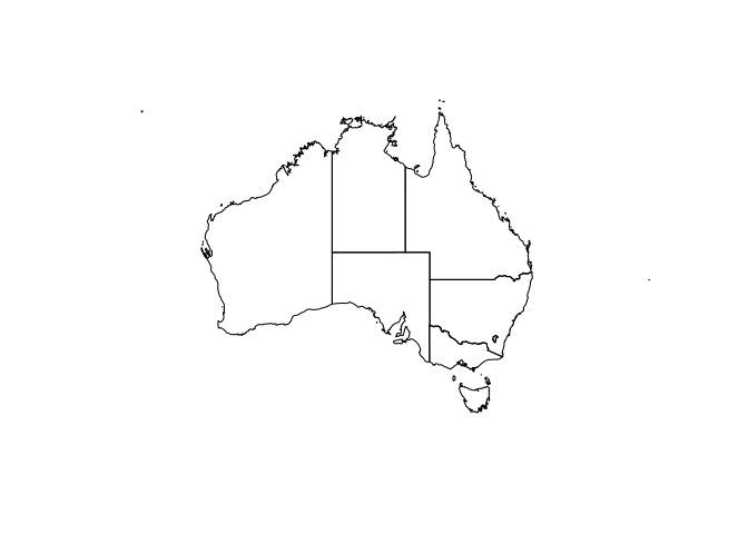
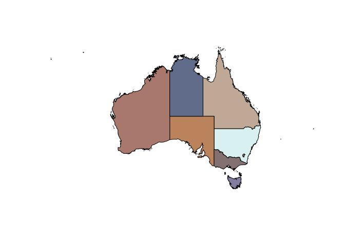
Plot Australia with states.
Plot Australia without states.
ozmap(x = "country")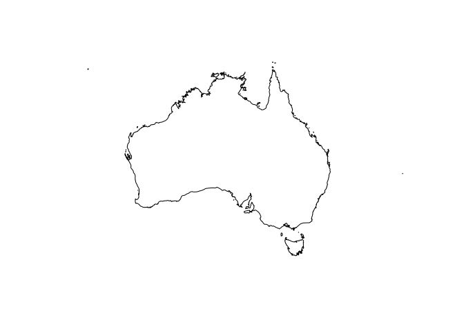
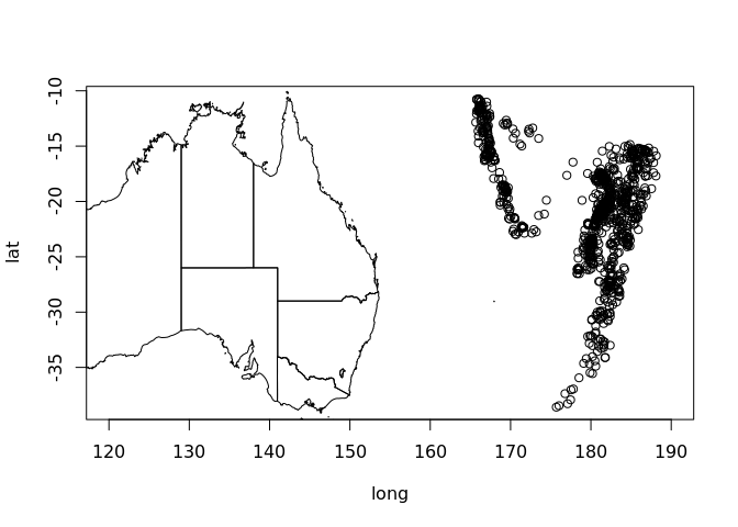
Add to an existing plot.
Obtain the data used in sf form.
sf_oz <- ozmap_data("states")

tibble::as_tibble(sf_oz)
#> # A tibble: 9 x 2
#>   NAME                                                                  geometry
#>   <chr>                                                       <MULTIPOLYGON [°]>
#> 1 New South Wales      (((150.7016 -35.12286, 150.6611 -35.11782, 150.6373 -35.…
#> 2 Victoria             (((146.6196 -38.70196, 146.6721 -38.70259, 146.6744 -38.…
#> 3 Queensland           (((148.8473 -20.3457, 148.8722 -20.37575, 148.8515 -20.3…
#> 4 South Australia      (((137.3481 -34.48242, 137.3749 -34.46885, 137.3805 -34.…
#> 5 Western Australia    (((126.3868 -14.01168, 126.3625 -13.98264, 126.3765 -13.…
#> 6 Tasmania             (((147.8397 -40.29844, 147.8902 -40.30258, 147.8812 -40.…
#> 7 Northern Territory   (((136.3669 -13.84237, 136.3339 -13.83922, 136.3532 -13.…
#> 8 Australian Capital … (((149.2317 -35.222, 149.2346 -35.24047, 149.2716 -35.27…
#> 9 Other Territories    (((167.9333 -29.05421, 167.9188 -29.0344, 167.9313 -29.0…
Plot with a custom palette.
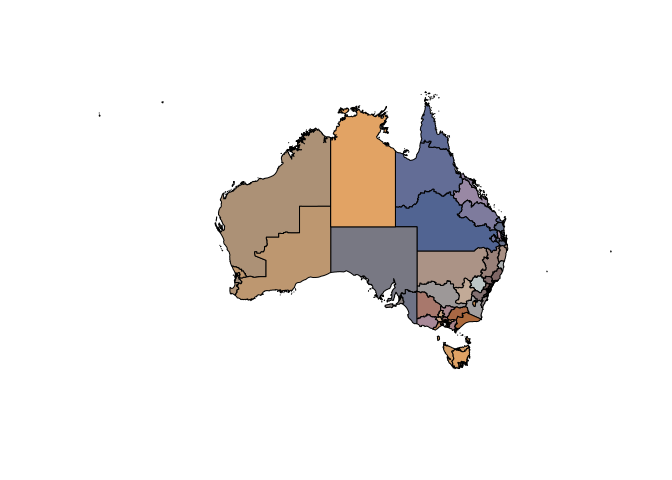
library(sf)
if (utils::packageVersion("paletteer") < '1.0.0') {
 pal <- paletteer::paletteer_d(package = "ochRe", palette = "namatjira_qual")
} else {
  pal <- paletteer::paletteer_d(palette = "ochRe::namatjira_qual")
}

opal <- colorRampPalette(pal)
nmjr <- opal(nrow(sf_oz))
plot(st_geometry(sf_oz), col = nmjr)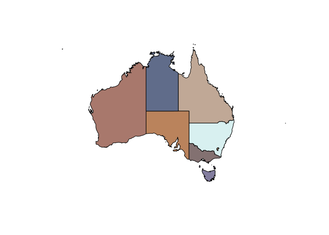
## plot directly with ggplot2
library(ggplot2)
ggplot(sf_oz, aes(fill = NAME)) + geom_sf() + coord_sf(crs = "+proj=lcc +lon_0=135 +lat_0=-30 +lat_1=-10 +lat_2=-45 +datum=WGS84") + scale_fill_manual(values = nmjr)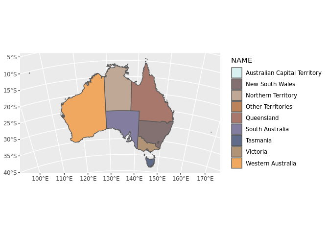
Plot the ABS layers (from 2016).
Resolution
These ABS layers abs_ced, abs_lga, and abs_ste are derived from the 2016 sources and simplified using rmapshaper::ms_simplify(, keep = 0.05, keep_shapes = TRUE) so all the original polygons are there. There is sufficient detail to map many (most?) of the regions on their own, which was a major goal for this package.
The cache of the source data at original resolution is available in ozmaps.data.
Compare the detail of Bruny Island here in this box, compared with the very basic maps package layer.
library(dplyr)
kbor <- abs_lga %>% dplyr::filter(grepl("Kingborough", NAME))
bb <- st_bbox(kbor)

layout(matrix(c(1, 1, 1, 2, 2, 2, 2, 2, 2), nrow = 3))
plot(kbor, reset = FALSE, main = "Kingborough (TAS)")
rect(bb["xmin"], bb["ymin"], bb["xmax"], bb["ymax"])
library(mapdata)
#> Loading required package: maps
par(mar = rep(0, 4))
plot(c(145, 148.5), c(-43.6, -40.8), type = "n", asp = 1/cos(mean(bb[c(2, 4)]) * pi/180), axes = FALSE, xlab = "", ylab = "")
maps::map(database = "worldHires", regions = "australia", xlim = c(145, 148.5), ylim = c(-43.6, -40.8), add = TRUE)
rect(bb["xmin"], bb["ymin"], bb["xmax"], bb["ymax"])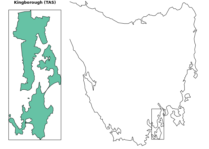
Please note that the ‘ozmaps’ project is released with a Contributor Code of Conduct. By contributing to this project, you agree to abide by its terms.