Bivariate Binning into Hexagon Cells

Creates a "hexbin" object. Basic components are a cell id and a count of points falling in each occupied cell.

Basic methods are show(), plot() and summary(), but also erode.

hexbin(x, y, xbins = 30, shape = 1,
       xbnds = range(x), ybnds = range(y),
       xlab = NULL, ylab = NULL, IDs = FALSE)

Arguments

x, y

vectors giving the coordinates of the bivariate data points to be binned. Alternatively a single plotting structure can be specified: see xy.coords. NA's are allowed and silently omitted.

xbins

the number of bins partitioning the range of xbnds.

shape

the shape = yheight/xwidth of the plotting regions.

xbnds, ybnds

horizontal and vertical limits of the binning region in x or y units respectively; must be numeric vector of length 2.

xlab, ylab

optional character strings used as labels for x and y. If NULL, sensible defaults are used.

IDs

logical indicating if the individual cell “IDs” should be returned, see also below.

Value

an S4 object of class "hexbin". It has the following slots:

cell

vector of cell ids that can be mapped into the (x,y) bin centers in data units.

count

vector of counts in the cells.

xcm

The x center of mass (average of x values) for the cell.

ycm

The y center of mass (average of y values) for the cell.

xbins

number of hexagons across the x axis. hexagon inner diameter =diff(xbnds)/xbins in x units

shape

plot shape which is yheight(inches) / xwidth(inches)

xbnds

x coordinate bounds for binning and plotting

ybnds

y coordinate bounds for binning and plotting

dimen

The i and j limits of cnt treated as a matrix cnt[i,j]

n

number of (non NA) (x,y) points, i.e., sum(* @count).

ncells

number of cells, i.e., length(* @count), etc

call

the function call.

xlab, ylab

character strings to be used as axis labels.

cID

of class, "integer or NULL", only if IDs was true, an integer vector of length n where cID[i] is the cell number of the i-th original point (x[i], y[i]). Consequently, the cell and count slots are the same as the names and entries of table(cID), see the example.

See also

hcell2xy gplot.hexbin, grid.hexagons, grid.hexlegend.

References

Carr, D. B. et al. (1987) Scatterplot Matrix Techniques for Large \(N\). JASA 83, 398, 424--436.

Details

Returns counts for non-empty cells only. The plot shape must be maintained for hexagons to appear with equal sides. Some calculations are in single precision.

Note that when plotting a hexbin object, the grid package is used. You must use its graphics (or those from package lattice if you know how) to add to such plots.

Examples

set.seed(101)
x <- rnorm(10000)
y <- rnorm(10000)
(bin <- hexbin(x, y))
#> 'hexbin' object from call: hexbin(x = x, y = y) 
#> n = 10000  points in	nc = 562  hexagon cells in grid dimensions  36 by 31 
## or
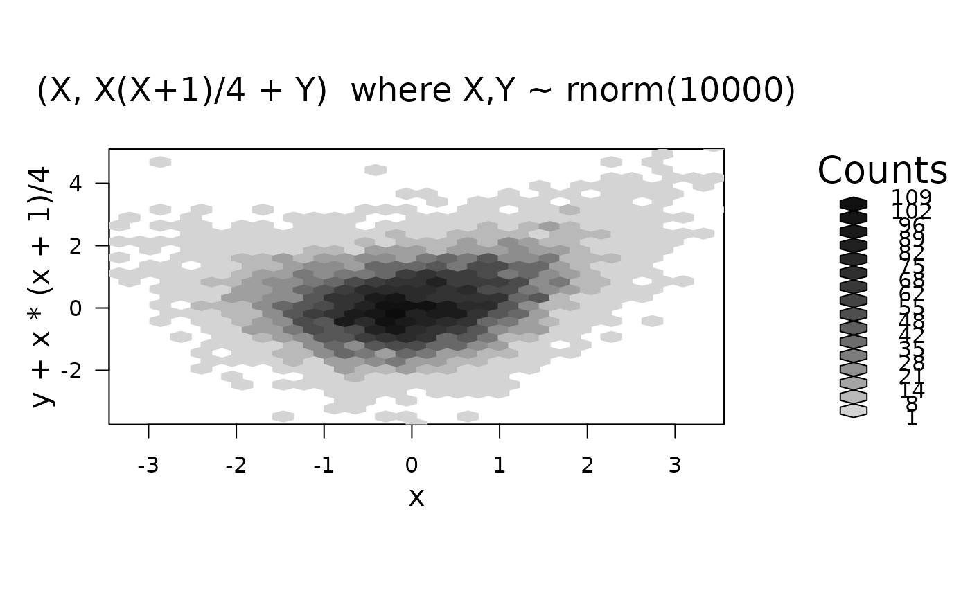
plot(hexbin(x, y + x*(x+1)/4),
     main = "(X, X(X+1)/4 + Y)  where X,Y ~ rnorm(10000)")


## Using plot method for hexbin objects:
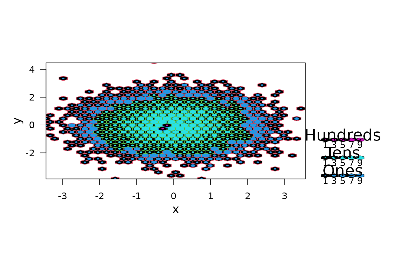
plot(bin, style = "nested.lattice")


hbi <- hexbin(y ~ x, xbins = 80, IDs= TRUE)
str(hbi)
#> Formal class 'hexbin' [package "hexbin"] with 16 slots
#>   ..@ cell  : int [1:2444] 48 103 202 284 445 522 698 720 747 759 ...
#>   ..@ count : int [1:2444] 1 1 1 1 1 1 1 1 1 1 ...
#>   ..@ xcm   : num [1:2444] 0.6777 -1.5365 -0.0576 0.06 0.0155 ...
#>   ..@ ycm   : num [1:2444] -3.88 -3.77 -3.72 -3.62 -3.38 ...
#>   ..@ xbins : num 80
#>   ..@ shape : num 1
#>   ..@ xbnds : num [1:2] -3.45 3.56
#>   ..@ ybnds : num [1:2] -3.88 4.47
#>   ..@ dimen : num [1:2] 94 81
#>   ..@ n     : int 10000
#>   ..@ ncells: int 2444
#>   ..@ call  : language hexbin(x = y ~ x, xbins = 80, IDs = TRUE)
#>   ..@ xlab  : chr "x"
#>   ..@ ylab  : chr "y"
#>   ..@ cID   : int [1:10000] 2061 2881 4163 4173 4012 4508 3206 3927 2805 3196 ...
#>   ..@ cAtt  : int(0) 
tI <- table(hbi@cID)
stopifnot(names(tI) == hbi@cell,
                tI  == hbi@count)

## NA's now work too:
x[runif(6, 0, length(x))] <- NA
y[runif(7, 0, length(y))] <- NA
hbN <- hexbin(x,y)
summary(hbN)
#> 'hexbin' object from call: hexbin(x = x, y = y) 
#> n = 9987  points in	nc = 562  hexagon cells in grid dimensions  36 by 31 
#>       cell            count             xcm                 ycm          
#>  Min.   :   9.0   Min.   :  1.00   Min.   :-3.449949   Min.   :-3.87679  
#>  1st Qu.: 352.2   1st Qu.:  2.00   1st Qu.:-1.257343   1st Qu.:-1.22151  
#>  Median : 515.5   Median :  7.00   Median :-0.005620   Median :-0.02137  
#>  Mean   : 517.5   Mean   : 17.77   Mean   :-0.001689   Mean   : 0.02506  
#>  3rd Qu.: 686.8   3rd Qu.: 24.00   3rd Qu.: 1.301911   3rd Qu.: 1.39114  
#>  Max.   :1098.0   Max.   :108.00   Max.   : 3.557626   Max.   : 4.47080