Add Hexagon Cells to Plot

Plots cells in an hexbin object. The function distinquishes among counts using 5 different styles. This function is the hexagon plotting engine from the plot method for hexbin objects.

grid.hexagons(dat, style = c("colorscale", "centroids", "lattice",
        "nested.lattice", "nested.centroids", "constant.col"),
         use.count=TRUE, cell.at=NULL,
   minarea = 0.05, maxarea = 0.8, check.erosion = TRUE,
   mincnt = 1, maxcnt = max(dat@count), trans = NULL,
   colorcut = seq(0, 1, length = 17),
   density = NULL, border = NULL, pen = NULL,
   colramp = function(n){ LinGray(n,beg = 90, end = 15) },
   def.unit=  "native",
   verbose = getOption("verbose"))

Arguments

dat: an object of class hexbin, see hexbin.
style: character string specifying the type of plotting; must be (a unique abbrevation) of the values given in ‘Usage’ above.
use.count: logical specifying if counts should be used.
cell.at: numeric vector to be plotted instead of counts, must besame length as the number of cells.
minarea: numeric, the fraction of cell area for the lowest count.
maxarea: the fraction of the cell area for the largest count.
check.erosion: logical indicating only eroded points should be used for "erodebin" objects; simply passed to hcell2xy, see its documentation.
mincnt: numeric; cells with counts smaller than mincnt are not shown.
maxcnt: cells with counts larger than this are not shown.
trans: a transformation function (or NULL) for the counts, e.g., sqrt.
colorcut: a vector of values covering [0, 1] which determine hexagon color class boundaries or hexagon size boundaries -- for style = "colorscale" only.
density: grid.polygon argument for shading. 0 causes the polygon not to be filled. This is not implemented (for grid.polygon) yet.
border: grid.polygon() argument. Draw the border for each hexagon.
pen: colors for grid.polygon(). Determines the color with which the polygon will be filled.
colramp: function of an integer argument n returning n colors. n is determined

def.unit: default unit to be used.

verbose: logical indicating if some diagnostic output should happen.

SIDE EFFECTS

Adds hexagons to the plot.

Details

The six plotting styles have the following effect:

style="lattice" or "centroids":

Plots the hexagons in different sizes based on counts. The "lattice" version centers the hexagons at the cell centers whereas "centroids" moves the hexagon centers close to the center of mass for the cells. In all cases the hexagons will not plot outside the cell unless maxarea > 1. Counts are rescaled into the interval [0,1] and colorcuts determine the class boundaries for sizes and counts. The pen argument for this style should be a single color or a vector of colors of length(bin@count).

style="colorscale":

Counts are rescaled into the interval [0,1] and colorcuts determines the class boundaries for the color classes. For this style, the function passed as colramp is used to define the n colors for the n+1 color cuts. The pen argument is ignored. See LinGray for the default colramp and alternative “color ramp” functions.

style="constant.col":

This is an even simpler alternative to "colorscale", using constant colors (determined pen optionally).

style="nested.lattice" and "nested.centroids":

Counts are partitioned into classes by power of 10. The encoding nests hexagon size within powers of 10 color contours.

If the pen argument is used it should be a matrix of colors with 2 columns and either ceiling(log10(max(bin@count))) or length(bin@count) rows. The default uses the R color palatte so that pens numbers 2-11 determine colors for completely filled cell Pen 2 is the color for 1's, Pen 3 is the color for 10's, etc. Pens numbers 12-21 determine the color of the foreground hexagons. The hexagon size shows the relative count for the power of 10. Different color schemes give different effects including 3-D illusions

Hexagon size encoding minarea and maxarea determine the area of the smallest and largest hexagons plotted. Both are expressed fractions of the bin cell size. Typical values might be .04 and 1. When both values are 1, all plotted hexagons are bin cell size, if maxarea is greater than 1 than hexagons will overlap. This is sometimes interesting with the lattice and centroid styles.

Count scaling

relcnt <- (trans(cnt)-trans(mincnt)) / (trans(maxcnt)-trans(mincnt))
area <- minarea + relcnt*maxarea

By default the transformation trans() is the identity function. The legend routine requires the transformation inverse for some options.

Count windowing mincnt and maxcnt Only routine only plots cells with cnts in [mincnts, maxcnts]

References

Carr, D. B. (1991) Looking at Large Data Sets Using Binned Data Plots, pp. 7--39 in Computing and Graphics in Statistics; Eds. A. Buja and P. Tukey, Springer-Verlag, New York.

Author

Dan Carr <dcarr@voxel.galaxy.gmu.edu>; ported and extended by Nicholas Lewin-Koh nikko@hailmail.net.

Examples

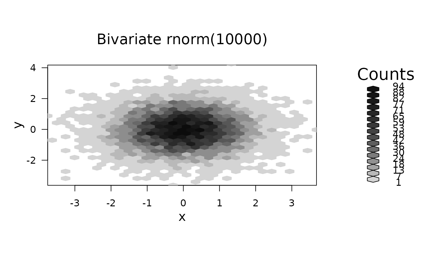
set.seed(506)
x <- rnorm(10000)
y <- rnorm(10000)

# bin the points
bin <- hexbin(x,y)

# Typical approach uses plot( <hexbin> ) which controls the plot shape :
plot(bin, main = "Bivariate rnorm(10000)")


## but we can have more manual control:

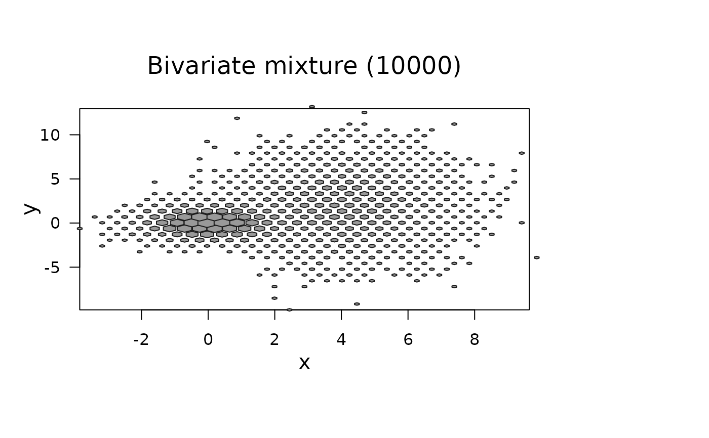
# A mixture distribution
x <- c(rnorm(5000),rnorm(5000,4,1.5))
y <- c(rnorm(5000),rnorm(5000,2,3))
hb2 <- hexbin(x,y)

# Show color control and overplotting of hexagons
## 1) setup coordinate system:
P <- plot(hb2, type="n", main = "Bivariate mixture (10000)")# asp=1

## 2) add hexagons (in the proper viewport):
pushHexport(P$plot.vp)
grid.hexagons(hb2, style= "lattice", border = gray(.1), pen = gray(.6),
              minarea = .1, maxarea = 1.5)
#> Warning: maxarea > 1, hexagons may overplot
library("grid")
popViewport()


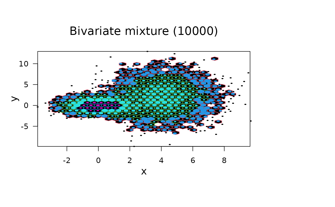
## How to treat 'singletons' specially:
P <- plot(hb2, type="n", main = "Bivariate mixture (10000)")# asp=1
pushHexport(P$plot.vp)
grid.hexagons(hb2, style= "nested.centroids", mincnt = 2)# not the single ones
grid.hexagons(hb2, style= "centroids", maxcnt = 1, maxarea=0.04)# single points
popViewport()