Spatial in ggsql: a guided tour
1. What ggsql is, in one query
ggsql is a SQL dialect with a plot grammar bolted onto the end of the query, and the thing to hold onto is that every statistic, join, filter and reprojection runs in the database, not in the plotting engine. The Rust core parses the query, rewrites it into backend SQL (DuckDB, SQLite, PostGIS, anything with ODBC or ADBC), pulls back only the rows the marks need as Arrow, and renders. It is by Thomas Lin Pedersen, Teun van den Brand and George Stagg at Posit, first alpha April 2026, beta (0.5.0) September 2026; the R package ggsql on CRAN wraps the same Rust library.
The grammar is ggplot2’s, with the vocabulary renamed so it reads as SQL. One query uses most of it:
SELECT * FROM ggsql:penguins
WHERE island = 'Biscoe'
VISUALISE bill_len AS x, bill_dep AS y, body_mass AS fill
DRAW point
PLACE rule
  SETTING slope => 0.4, y => -1
SCALE BINNED fill
FACET species
PROJECT TO cartesian
LABEL title => 'Bill dimensions', x => 'Bill length (mm)'| ggsql clause | ggplot2 equivalent | what it does |
|---|---|---|
VISUALISE a AS x, b AS y [FROM t] |
ggplot(t, aes(x = a, y = b)) |
global mappings and the data source; ggsql:penguins is a built-in dataset |
DRAW point |
geom_point() |
a layer; takes MAPPING, REMAPPING (stat outputs), SETTING (constants and parameters), FILTER (a WHERE for this layer), PARTITION BY (group), ORDER BY, in that order |
PLACE rule SETTING ... |
annotate() |
a layer with no data source, placed by constants |
SCALE BINNED fill TO magma VIA log10 |
scale_fill_binned(...) + transform |
scale type, palette, transform, breaks |
FACET species |
facet_wrap(~species) |
small multiples |
PROJECT x, y TO cartesian |
coord_*() |
the coordinate system; cartesian, polar, and the map projections below |
LABEL title => '...' |
labs() |
titles, axis labels, captions, with markdown |
Three things differ from ggplot2 and matter for spatial work. There is no stat/geom split: a layer is one thing, and summaries come from an aggregate setting on the layer (SETTING aggregate => 'mean') that collapses each group in SQL. PARTITION BY is group, and ORDER BY is arrange, both on the layer, so the “group then arrange” construction of a line or a polygon from a vertex table is first-class syntax. And PROJECT is where the coordinate system lives, with the aesthetic names chosen by the coord: a map coord’s primary and secondary aesthetics are lon and lat, and PROJECT x, y TO map renames them.
The pipeline, for a query with a projection, is:
- Parse, resolve mappings and scales, decide the coord.
- Build one SQL query per layer: the user’s query as a subquery, plus the layer’s filter, aggregation, densification and (for a map)
ST_Transform. - Materialise each layer to a temp table, compute bounding boxes in SQL.
- Fetch the rows as Arrow and hand them to the writer:
hephaestus, the new vector/raster renderer (SVG, PDF, PNG and friends), or Vega-Lite as a legacy writer.
So “the plot is the collect” still holds, as in ggplot2, but the collect is as small as the marks allow, and everything before it is pushed down. That is the design decision that makes spatial interesting here.
2. How spatial works inside ggsql
ggsql knows about projections but never evaluates one: every coordinate transform is ST_Transform in the database, and the Rust side’s job is to decide what the visible area is and to draw it. That is the whole architecture, and it is worth seeing the pieces (ggsql 0.5.2, src/plot/projection/coord/map.rs, map_projections.rs, src/plot/layer/geom/spatial.rs).
The spatial layer. DRAW spatial takes one required aesthetic, geometry, which it auto-detects from the column names. The contract is simple features in WKB: whatever the backend can hand over through ST_AsWKB (DuckDB) or ST_AsBinary (PostGIS, SpatiaLite; SQL Server has its own) works. Tested backends are DuckDB spatial, PostGIS and SpatiaLite. The built-in ggsql:world is Natural Earth 110m countries, stored as GeoParquet and registered into DuckDB with the geometry already converted to WKB.
Source CRS. Before projecting, ggsql runs ST_SRID on the geometry column. A non-zero SRID becomes EPSG:<srid>; zero or absent falls back to the source setting, which defaults to EPSG:4326. Remember this: WKB carries no SRID, so anything you have already projected and handed over as WKB will be assumed to be longitude/latitude unless you say otherwise.
Target CRS and the 21 named projections. PROJECT TO robinson or PROJECT TO crs SETTING target => 3031 both resolve to a PROJ string. The named ones are hand-written structs in Rust (orthographic, stereographic, gnomonic, Lambert azimuthal, azimuthal equidistant, Mercator, transverse Mercator, UTM, Miller, equirectangular, cylindrical equal-area, Mollweide, sinusoidal, Eckert IV, Natural Earth, Winkel tripel, Albers, Lambert conformal conic, Goode homolosine, Robinson, Equal Earth), and a small parser maps a PROJ string or a known EPSG code (4326, 3031, 3413, 3395, 9354, UTM zones) back onto one of them. What those structs provide is not a transform. Each one answers two questions: what does the horizon look like, as a polygon in longitude/latitude (a hemisphere ring of 88 degrees for orthographic, 60 for gnomonic, a world box for the pseudocylindricals, and so on), and which PROJ parameters do origin and parallel map to.
What happens to a layer under a map coord. For the spatial layer: the horizon polygon is sent to the database as WKT, ST_Transformed, and used in ST_Intersection to clip the geometry, then ST_Transform to the target, then ST_AsWKB back. For a non-spatial layer with position aesthetics (path, polygon, point, text, rect, tile): the edges are densified in SQL by linear interpolation in source units (segments longer than one degree get intermediate vertices), then ST_Transform. No horizon clip is applied to these. Every projected layer is materialised to a temp table and its bounding box computed there, which is how the panel knows its extent without the data leaving the database.
Rendering. Rows come back as Arrow with a binary WKB column. geozero decodes it, and the writer draws it. The new renderer (hephaestus) takes WKB and WKT natively, fills polygons with holes correctly, and meshes variable-width lines into triangles rather than chopping them into segments. The grey panel background under a map is the horizon polygon again, this time drawn.
So the division of labour is: PROJ, via the database’s spatial extension, does geodesy; ggsql’s Rust knows enough cartography to clip at the horizon and draw the panel; the renderer knows simple features. Nothing in the Rust tree depends on a geometry or projection library, and that is a deliberate choice. It also means that anything the spatial extension can do in SQL (ST_Intersects in a FILTER, a LEFT JOIN on a reference table, ST_Simplify) is available to the user without ggsql knowing about it, and that is where the rest of this document lives.
3. Route 1: the WKB spatial layer
The advertised path works well, including at the pole, and the one artefact it shows is in the data. Everything in this section is two or three lines of ggsql against the built-in dataset.
VISUALISE continent AS fill FROM ggsql:world
DRAW spatial
PROJECT TO robinson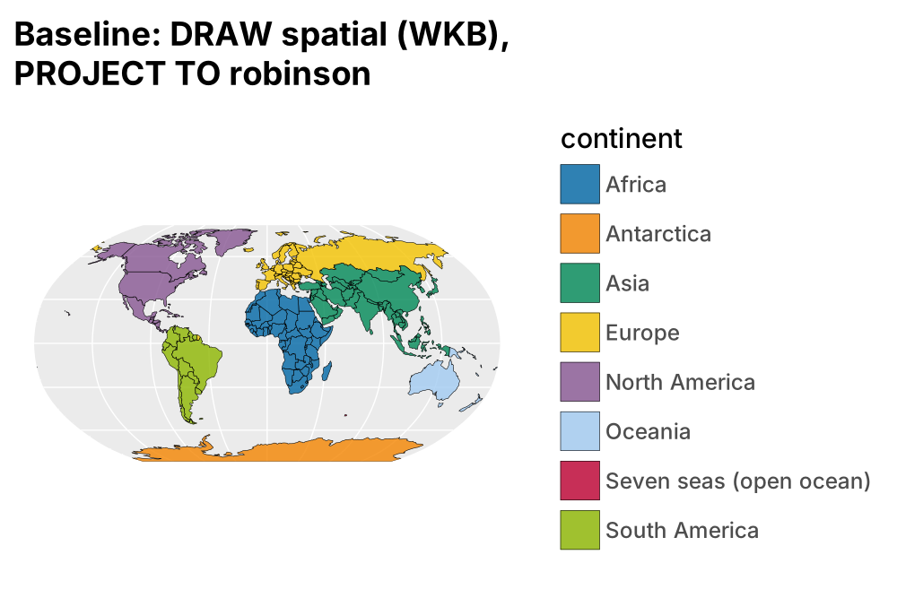
A polar view is a named projection with an origin, or an EPSG code. These two queries produce the same figure, because ggsql recognises 3031 as +proj=stere +lat_0=-90 and gives it the stereographic horizon treatment.
PROJECT TO stereographic SETTING origin => (0, -90)
-- or
PROJECT TO crs SETTING target => 3031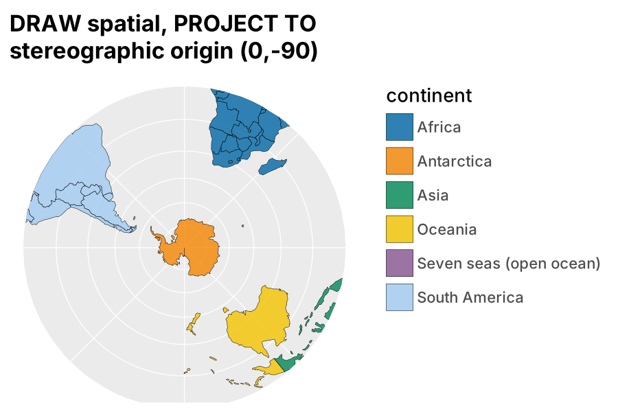
The horizon is an 88-degree cap around the antipode, so everything north of about 2 degrees south is clipped away in SQL before it is drawn, and the panel is the circle. bounds zooms, in target units (metres here):
PROJECT TO crs SETTING target => 3031, bounds => (-5500000, -5500000, 5500000, 5500000)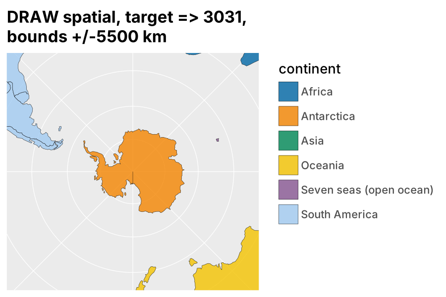
The vertical line from the pole is not a ggsql bug. Natural Earth’s Antarctica ring runs down the 180 meridian to latitude -90 and back up the -180 meridian, so in any polar projection the two edges land on the same ray and the renderer strokes a zero-width slit. It is in ggsql:world and in every example on ggsql.org that shows Antarctica; section 5 removes it.
Holes are handled: the renderer fills WKB polygons with the correct rule, so Lesotho’s hole in South Africa shows through without anyone thinking about it.
VISUALISE name AS fill FROM ggsql:world
DRAW spatial
  FILTER name IN ('South Africa', 'Eswatini', 'Namibia', 'Botswana')
PROJECT TO geographic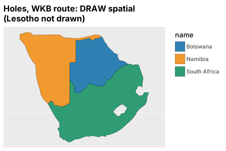
Two practical notes. The spatial extension must be loadable by the backend; with the DuckDB reader a leading LOAD spatial; statement in the query is the portable way, and for the spatial layer ggsql triggers the autoload itself. And DRAW spatial has no settings of its own, so detail, simplification and selection all happen in the SQL above the VISUALISE line, which is the point.
4. Route 2: the vertex table
Group plus arrange is how the grammar of graphics has always built a line, and it builds a polygon the same way; ggsql has both operations on the layer, so the vertex-table route works today and needs two small things to be complete. This is the route that matters for anyone whose polygons are not simple features: anatomy diagrams, sports fields, teeth, or a coastline you built from segments.
The table is one row per vertex, with the identity of the feature, the part and the ring, and the order within the ring. From ggsql:world that is 10,654 rows (data/world_vertices.parquet):
| fid | name | poly | ring | is_hole | ord | x | y |
|---|---|---|---|---|---|---|---|
| 158 | Antarctica | 0 | 0 | false | 0 | 180.0 | -84.713 |
| 158 | Antarctica | 0 | 0 | false | 1 | 180.0 | -90.0 |
| 158 | Antarctica | 0 | 0 | false | 2 | -180.0 | -90.0 |
| 158 | Antarctica | 0 | 0 | false | 3 | -180.0 | -84.713 |
The plot is the polygon layer, partitioned by feature, part and ring, ordered by vertex:
LOAD spatial;
VISUALISE x AS lon, y AS lat, continent AS fill FROM 'world_vertices.parquet'
DRAW polygon
  PARTITION BY fid, poly, ring
  ORDER BY ord
PROJECT TO stereographic SETTING origin => (0, -90)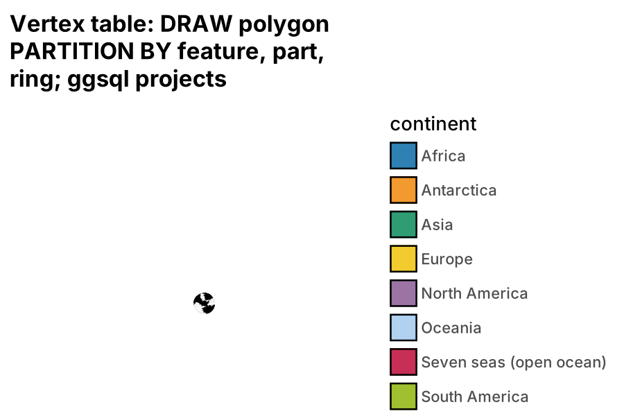
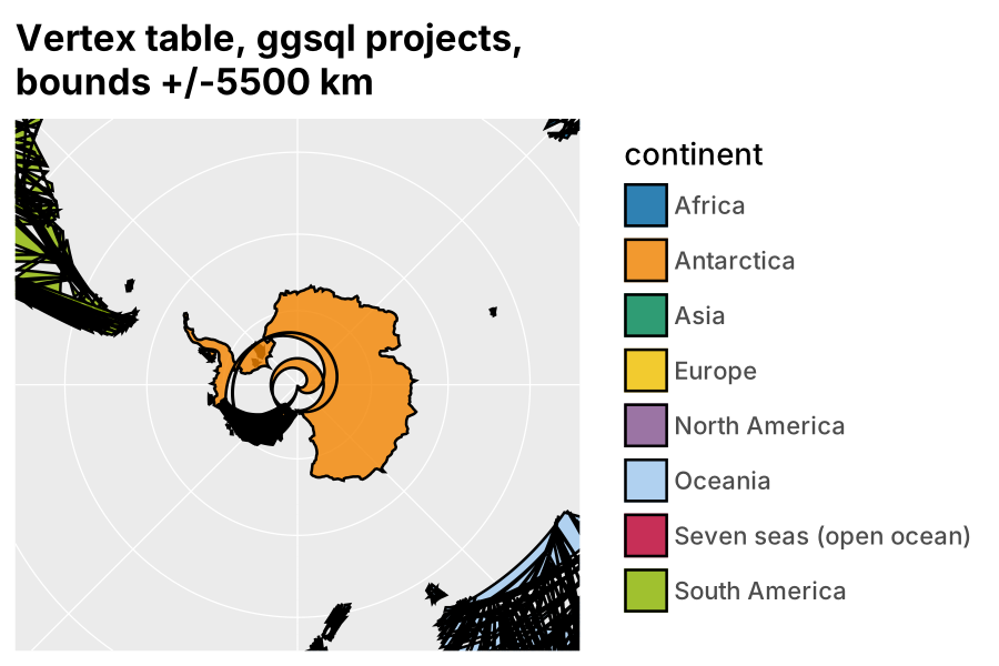
The globe is tiny because nothing was clipped. The spatial layer gets the horizon intersection; a polygon layer gets densified and transformed, and a vertex at 60 degrees north projects to a hundred million metres under south polar stereographic, so the panel autoscales to that. With bounds the view is right but the unclipped edges wrap through it:
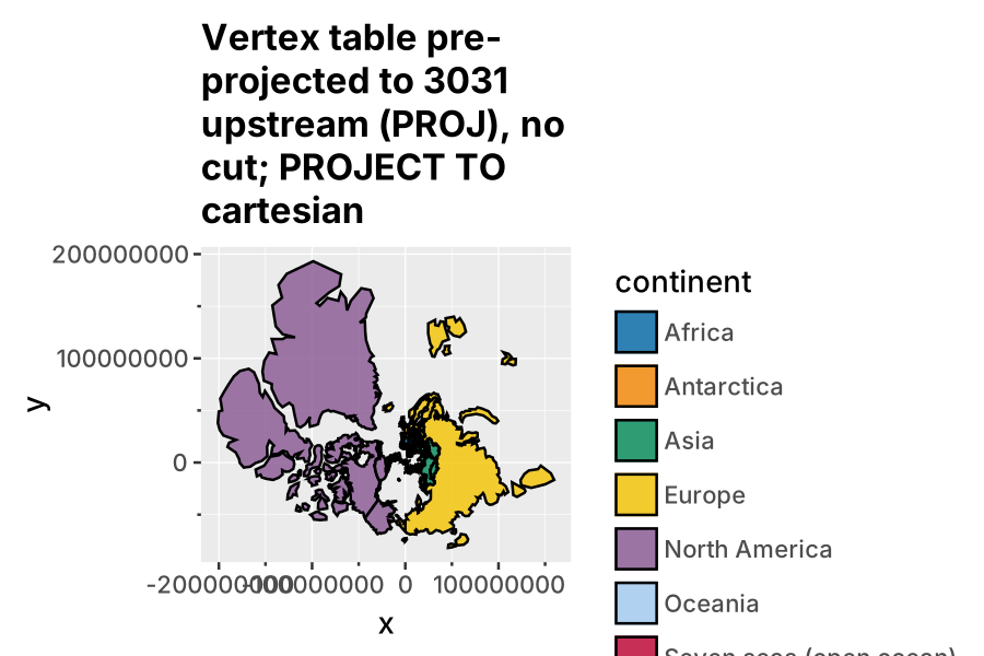
Pre-projecting the table yourself (PROJ in R or Python, section 5) and drawing it in cartesian gives a correct whole-plane south polar stereographic: nothing is wrong with it, the north pole is at infinity and Natural Earth’s northernmost vertices sit at a hundred million metres, so the autoscaled panel is the whole plane:
A view is a scale range, not a cut. SCALE x FROM (...) and SCALE y FROM (...) set the window in target units, ratio => 1 keeps metres square, and the cartesian coord clips at the panel edge:
VISUALISE x, y, continent AS fill FROM 'world_3031.parquet'
DRAW polygon
  PARTITION BY fid, poly, ring
  ORDER BY ord
SCALE x FROM (-5500000, 5500000)
SCALE y FROM (-5500000, 5500000)
PROJECT TO cartesian SETTING ratio => 1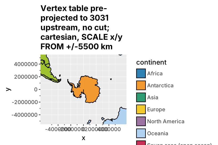
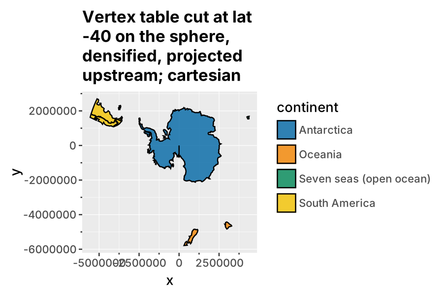
What the upstream cut buys is not the view but the geometry: a ring cut on the sphere around the pole has no antimeridian seam, densification before projection gives the edges their curvature, and the legend only carries what is on the map. Cut first, with a ring around the pole rather than a bounding box, densify, then project:
Holes
A hole is a ring with ring > 0. Partition by ring and each ring is its own polygon, so the hole fills over the exterior (Lesotho here is a darker green patch, not a gap):
DRAW polygon
  FILTER name IN ('South Africa', 'Eswatini', 'Namibia', 'Botswana')
  PARTITION BY fid, poly, ring
  ORDER BY ord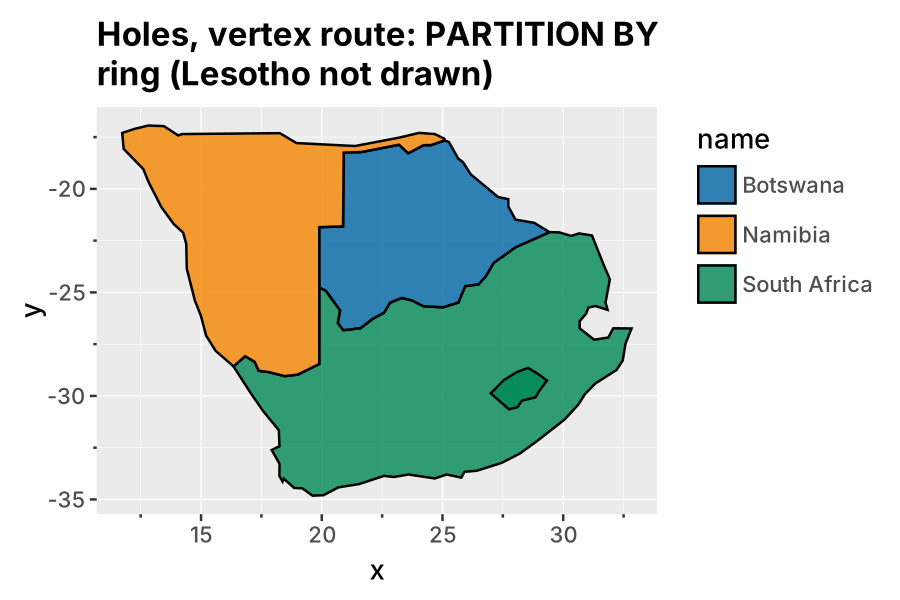
Partition by feature only, ordering by part, ring and vertex, and the renderer’s winding rule produces the hole, plus a stroke along the edge that joins the exterior to the interior ring. That is ggpolypath from 2016, in a new renderer:
DRAW polygon
  FILTER name IN ('South Africa', 'Eswatini', 'Namibia', 'Botswana')
  PARTITION BY fid
  ORDER BY poly, ring, ord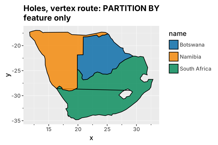
The fix is small: a polygon layer that knows a ring column (or a hole aesthetic), fills even-odd and does not stroke the join. The renderer already does exactly this for WKB input, so it is plumbing.
The spiral
The spiral in figure 10b is a bug, and a good one because it teaches the densification rule. Antarctica alone, PARTITION BY poly ORDER BY ord, is clean:
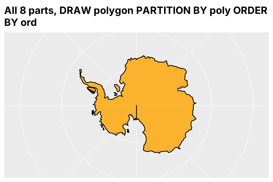
Add continent AS fill and the spiral appears:
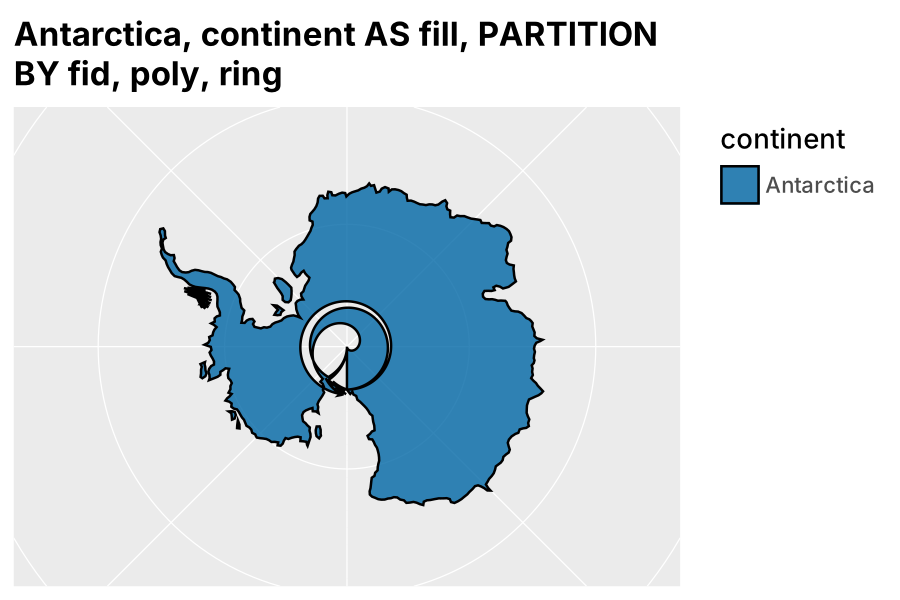
In the source, execute/layer.rs appends the layer’s ORDER BY to the layer query, and densify_edges in plot/layer/geom/mod.rs then wraps that query and numbers edges with ROW_NUMBER() OVER (PARTITION BY <partition columns and discrete mappings> ORDER BY (SELECT NULL)). The edge order is therefore whatever the window operator returns within each partition, and a discrete mapping changes the partition key set, so a few rows at the slit swap places. The resulting edge runs from (-180, -90) to (180, -84.7): linear interpolation in longitude and latitude sweeps 360 degrees while latitude climbs five, and under an azimuthal projection that is an Archimedean spiral. The fix is to use the layer’s ORDER BY as the window order.
The rule itself, with correct ordering, is shown by dropping the two pole vertices so the ring closes across the slit at -84.7 degrees:
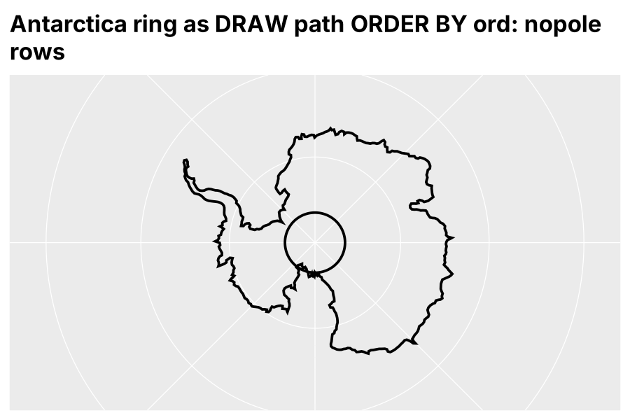
Linear densification in source coordinates is only safe on rings that have already been cut at the horizon and at the antimeridian. That is the one sentence to carry into section 5.
5. Route 3: prepare upstream
Everything ggsql cannot do for a map is three lines of wk, PROJ and geos, and the result is a table ggsql already draws; the one thing to know is the source => setting. This is the route to document, because it adds nothing to ggsql and it is how real data arrives anyway: cut to the region of interest, in the projection the analysis uses.
The preparation, in R (prep/recipe.R; the figures were produced by the same steps in pyproj and shapely, prep/prep.py and prep/prep_geoparquet.py, because the demo machine had no R, and it is the same PROJ underneath):
library(wk); library(PROJ); library(geos)
world <- arrow::read_parquet("world.parquet")
geom  <- wk::wkb(world$geom, crs = "OGC:CRS84")

# 1. cut on the sphere with a ring around the pole, so there is no antimeridian seam
horizon <- wk::wkt("POLYGON ((-180 -40, 180 -40, 180 -90, -180 -90, -180 -40))", crs = "OGC:CRS84")
cut <- geos::geos_intersection(geos::as_geos_geometry(geom), geos::as_geos_geometry(horizon))

# 2. densify so edges curve, then transform with PROJ
cut <- geos::geos_densify(cut, 1)
cut <- wk::wk_transform(wk::as_wkb(cut), PROJ::proj_trans_create("OGC:CRS84", "EPSG:3031"))

# 3. (data fix) Natural Earth's Antarctica slit: snap to 1 m, zero-width buffer
ant <- world$name == "Antarctica"
cut[ant] <- geos::as_geos_geometry(cut[ant]) |> geos::geos_set_precision(1) |> geos::geos_buffer(0) |> wk::as_wkb()

# either a vertex table...
vert <- cbind(world[wk::wk_coords(cut)$feature_id, c("name", "continent")], wk::wk_coords(cut))
# ...or WKB in a GeoParquet with CRS EPSG:3031
Three things in that recipe are the actual content. The horizon for a polar view is a ring around the pole, never a bounding box, because a box has edges at longitude 180 and -180 and those become a seam. Densify before you transform, so that an edge which is straight in longitude/latitude becomes the curve it should be in the target. And the slit is in the data, not the plot: in EPSG:3031 the two antimeridian edges differ by about 1e-10 m, so snapping to a metre and then a zero-width buffer dissolves it.
Handing it to ggsql
The prepared WKB goes through the spatial layer. The first attempt, a GeoParquet whose geometry column carries the CRS, fails in ggsql 0.5.2: ggsql emits ST_GeomFromWKB(CAST(geom AS BLOB)) and DuckDB 1.5 refuses to cast a typed GEOMETRY('<projjson>') column to a blob. The built-in dataset avoids this because ggsql converts it to WKB when it registers it. The user workaround is to do the same in the query, and once the geometry is WKB its SRID is gone, so ggsql assumes 4326 and transforms metres as degrees:
SELECT name, continent, population, ST_AsWKB(geom) AS geom FROM 'world_3031_cut_geo.parquet'
VISUALISE continent AS fill
DRAW spatial
PROJECT TO crs SETTING target => 3031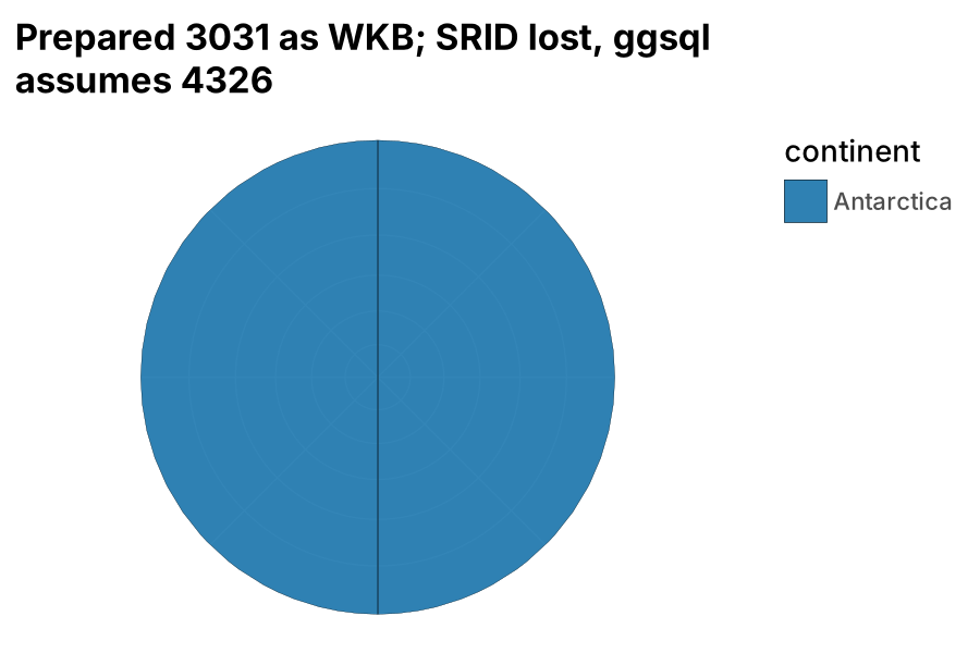
Declaring the source is the whole fix, and it is the recipe for any pre-projected data:
SELECT name, continent, population, ST_AsWKB(geom) AS geom FROM 'world_3031_cut_geo.parquet'
VISUALISE continent AS fill
DRAW spatial
PROJECT TO crs SETTING source => 'EPSG:3031', target => 3031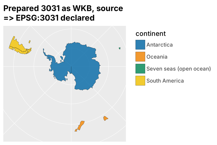
With source and target equal, ST_Transform is a no-op, ggsql still knows it is a stereographic map (3031 is in its table), so the horizon, the graticule and the panel are drawn, and the clipping has already been done upstream. PROJECT TO cartesian also works, with a plain grid instead of a graticule:
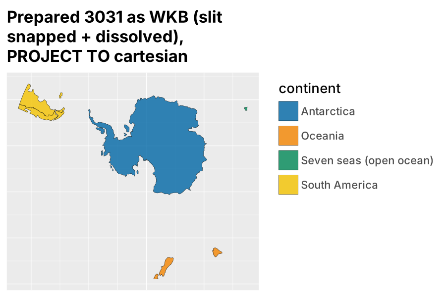
The same preparation serves the vertex route (figure 12) with PROJECT TO cartesian and no LOAD spatial at all, which is the smallest possible footprint: a Parquet file of x, y and ids, and a polygon layer.
What this gives a ggsql user is a division that matches the architecture in section 2: PROJ and GEOS do geodesy and topology once, upstream, where the user has the full toolkit; ggsql does what it is for, which is the grammar, the scales and the rendering, with the database doing the joins and filters in between.
6. Findings, and where this meets the wider thread
Seven items for posit-dev/ggsql, none of which needs a dependency on either side. The two bugs are each a few lines; the rest is documentation.
| # | kind | item | evidence |
|---|---|---|---|
| 1 | bug | CAST(geom AS BLOB) fails on DuckDB 1.5 for a GeoParquet with a non-trivial CRS; ST_AsWKB(geom) works everywhere ggsql already uses it |
section 5, first attempt |
| 2 | bug | layer ORDER BY is not propagated into densify_edges; path/polygon edge order under a map coord depends on engine row order within the partition |
figures 32 vs 33 |
| 3 | docs | source => is the escape hatch for pre-projected WKB; ST_AsWKB plus source is the recipe |
figures 13a, 13b |
| 4 | docs | a polar example (target => 3031, origin => (0, -90)) and a worked prepare-upstream example; the crs page’s region table has Antarctica under azimuthal_equidistant, and 3031 is what people use |
section 3 |
| 5 | docs | state the densification rule: linear in source units, so cut at horizon and antimeridian first | figure 30 |
| 6 | feature | ring/hole support in DRAW polygon (even-odd fill, no join stroke), so the vertex route is complete |
figures 21, 22 |
| 7 | feature | horizon-clip non-spatial layers under a map coord, as the spatial layer already is | figures 10, 10b |
And one observation for the built-in data: a snapped zero-width buffer on Antarctica at build time removes the slit from every example on the site.
The extension-club thread
The discussion at ggplot2-extenders/ggplot-extension-club#149 (Eva Maerey, Teun van den Brand, June to October 2026) runs on the same ground from the ggplot2 side, and the three routes here map onto its proposals directly.
Teun’s geometry scale (posit-dev/ggsql#453, ggplot2 PR #6896) maps names to shapes from a reference set, with detail level as a palette property. In ggsql a palette is a reference table and the scale is a join; the 0.4.1 release already shows LEFT JOIN world ON country = name. Route 3 is the same object from the other side: a reference set you have cut, densified and projected for the view you want, handed over with source => so ggsql leaves it alone. Detail as a palette property is a level-of-detail question, which belongs to an arc table or a coverage simplifier, not a renderer.
Eva’s bring-your-own-polygon packages (ggregions without sf, ggcolonviz’s part aesthetic, teethr) are route 2: a vertex table with a part column. Both those and the ggsql vertex route are complete once a polygon layer knows a ring. Her Alaska and Hawaii question (moved or projected?) is route 3 again: a per-feature transform with a different CRS per group and an affine shift is three lines, and the layer never needs to know.
The triangulation thread (trianglewins, barycentric interpolation on a mesh, the SOAP-film heatmap) is one step past route 2. hephaestus already meshes variable-width lines into triangles; a mesh layer taking a triangle table with a value per vertex is the vertex table one step further, and in ggsql the nearest thing today is tile. That is where ggsql’s vertex route and the mesh packages meet.
The framing to take into #336 is that the vertex route is not a workaround for people without sf. It is the general case, and the WKB spatial layer is a convenience on top of it. Teun’s scale and Eva’s examples both land there.
7. Appendix: reproducing everything
All figures came from one CLI binary and one shell script; see the README for the build and extension setup.
Rendering. queries/render.sh NAME "QUERY" runs ggsql exec --output figures/NAME.svg "QUERY" and rasterises the SVG to PNG with cairosvg. Clause order inside DRAW matters and the parser error is unhelpful: MAPPING, REMAPPING, SETTING, FILTER, PARTITION BY, ORDER BY.
Data. data/world.parquet is a copy of ggsql’s built-in dataset (src/data/world.parquet, Natural Earth 110m, GeoParquet with CRS OGC:CRS84). prep/prep.py decomposes it to the three vertex tables (world_vertices.parquet, world_3031.parquet, world_3031_cut.parquet); prep/prep_geoparquet.py writes world_3031_cut_geo.parquet, the cut and projected WKB with a PROJJSON CRS; prep/recipe.R is the same preparation in wk, PROJ and geos, written without an R session to hand, so check the function names before pasting into docs. data/ant_ring_*.parquet are the single-ring tests behind figures 30 to 34.
Queries by figure.
| figure | route | query (abbreviated) |
|---|---|---|
| 00 | 1 | DRAW spatial PROJECT TO robinson |
| 01, 02 | 1 | PROJECT TO stereographic SETTING origin => (0, -90) / PROJECT TO crs SETTING target => 3031 |
| 03 | 1 | target => 3031, bounds => (-5500000, -5500000, 5500000, 5500000) |
| 20 | 1 | southern Africa, PROJECT TO geographic |
| 10, 10b | 2 | world_vertices.parquet, DRAW polygon PARTITION BY fid, poly, ring ORDER BY ord, stereographic |
| 11, 11b | 2 | world_3031.parquet, same layer, PROJECT TO cartesian; 11b adds SCALE x FROM (-5500000, 5500000), same for y, ratio => 1 |
| 12 | 2 | world_3031_cut.parquet, same layer, PROJECT TO cartesian |
| 21, 22 | 2 | southern Africa from the vertex table, PARTITION BY fid, poly, ring / PARTITION BY fid |
| 30 | 2 | ant_ring_nopole.parquet, DRAW path ORDER BY ord |
| 32, 33 | 2 | Antarctica from the vertex table, PARTITION BY poly ORDER BY ord, without / with continent AS fill |
| 13a, 13b, 13c | 3 | SELECT ..., ST_AsWKB(geom) AS geom FROM 'world_3031_cut_geo.parquet', target => 3031 / source => 'EPSG:3031', target => 3031 / cartesian |
Sources. ggsql on CRAN - posit-dev/ggsql - issue 336, Spatial plotting - ggsql 0.4.1: spatial plotting - ggsql 0.5.0: readers, writers, beta - Spatial layer docs - Map coord docs - ggplot-extension-club discussion 149